Spatial Filtering to Enhance Low and High Frequency

Spatial Filtering to Enhance Low- and High -Frequency Detail and Edges A characteristics of remotely sensed images is a parameter called spatial frequency, defined as the number of changes in brightness value per unit distance for any particular part of an image.

Spatial Filtering to Enhance Low- and High -Frequency Detail and Edges Spatial frequency in remotely sensed imagery may be enhanced or subdued using two different approaches: - Spatial convolution filtering based primarily on the use of convolution masks, and - Fourier analysis which mathematically separates an image into its spatial frequency components.

Spatial Convolution Filtering A linear spatial filter is a filter for which the brightness value (BVi, j, out) at location i, j in the output image is a function of some weighted average (linear combination) of brightness values located in a particular spatial pattern around the i, j location in the input image. The process of evaluating the weighted neighboring pixel values is called two-dimensional convolution filtering.

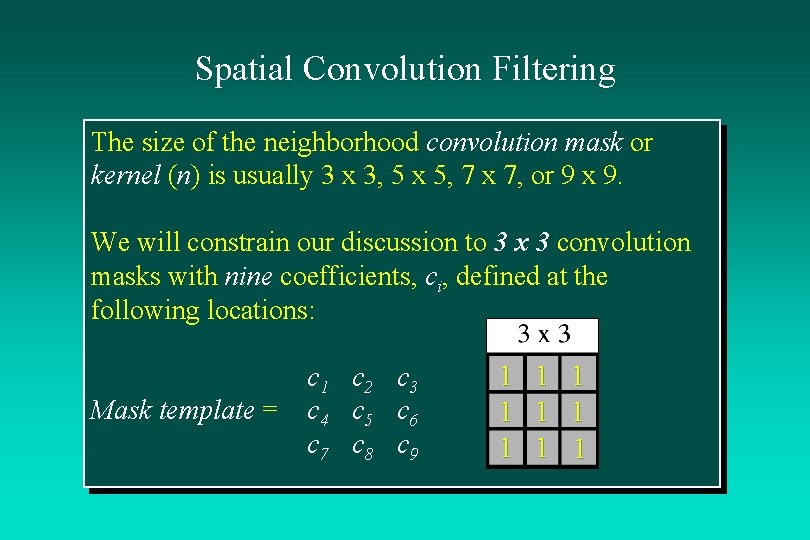
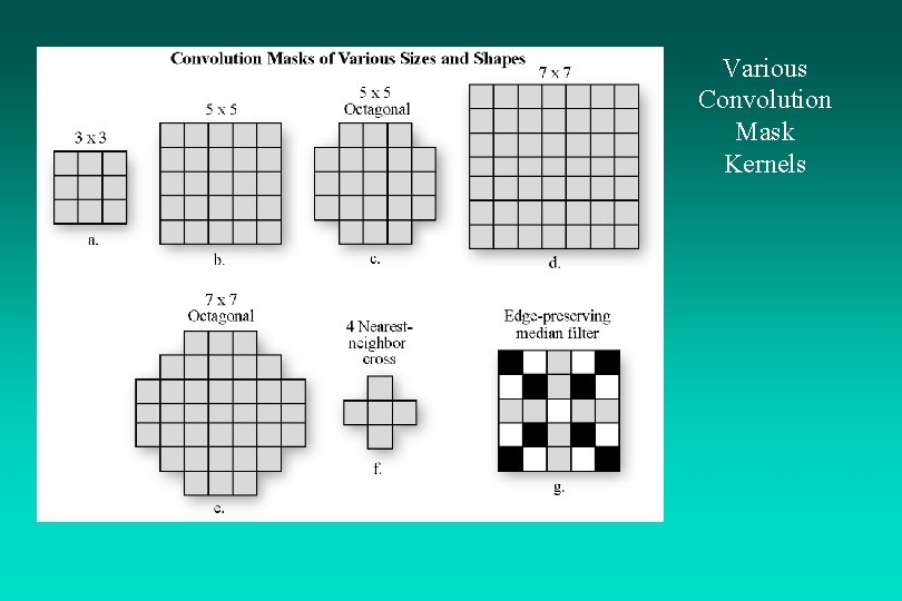
Spatial Convolution Filtering The size of the neighborhood convolution mask or kernel (n) is usually 3 x 3, 5 x 5, 7 x 7, or 9 x 9. We will constrain our discussion to 3 x 3 convolution masks with nine coefficients, ci, defined at the following locations: Mask template = c 1 c 4 c 7 c 2 c 5 c 8 c 3 c 6 c 9 1 1 1 1 1

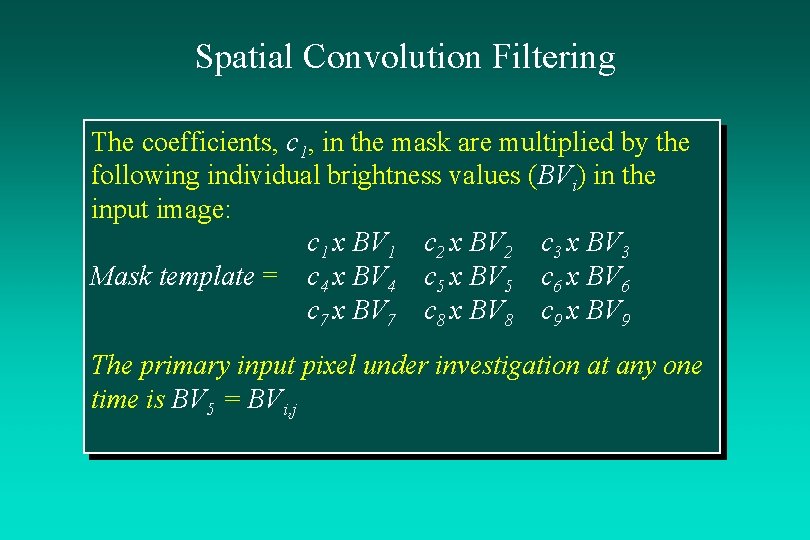
Spatial Convolution Filtering The coefficients, c 1, in the mask are multiplied by the following individual brightness values (BVi) in the input image: c 1 x BV 1 c 2 x BV 2 c 3 x BV 3 Mask template = c 4 x BV 4 c 5 x BV 5 c 6 x BV 6 c 7 x BV 7 c 8 x BV 8 c 9 x BV 9 The primary input pixel under investigation at any one time is BV 5 = BVi, j

Various Convolution Mask Kernels

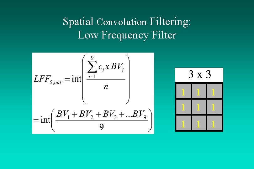
Spatial Convolution Filtering: Low Frequency Filter 1 1 1 1 1

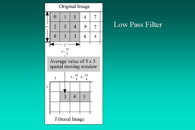
Low Pass Filter

Spatial Frequency Filtering

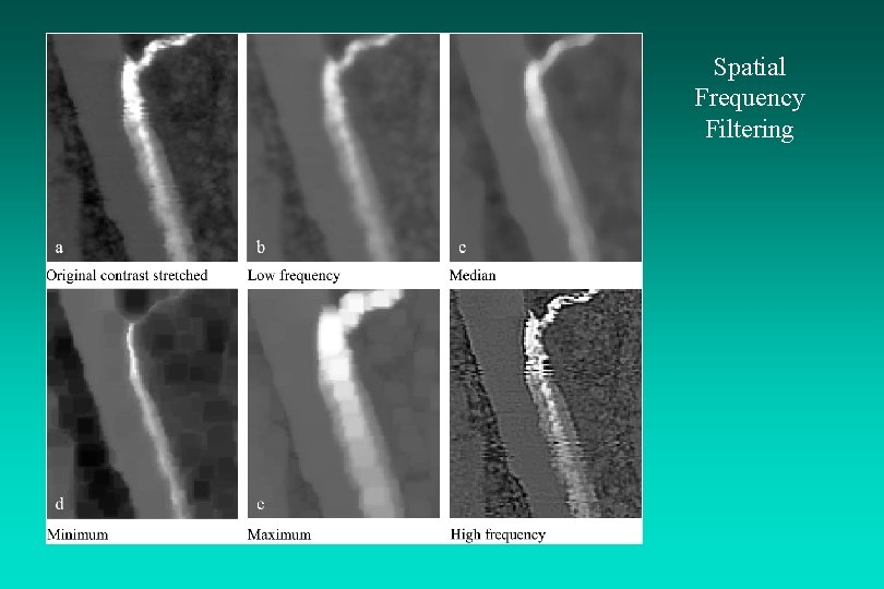
Spatial Filtering: Median Filter A median filter has certain advantages when compared with weighted convolution filters, including: 1) it does not shift boundaries, and 2) the minimal degradation to edges allows the median filter to be applied repeatedly which allows fine detail to be erased and large regions to take on the same brightness value (often called posterization).

Spatial Frequency Filtering

Spatial Filtering: Minimum or Maximum Filters Operating on one pixel at a time, these filters examine the brightness values of adjacent pixels in a userspecified radius (e. g. , 3 x 3 pixels) and replace the brightness value of the current pixel with the minimum or maximum brightness value encountered, respectively.

Spatial Frequency Filtering

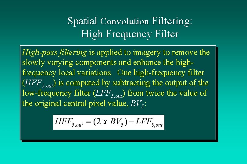
Spatial Convolution Filtering: High Frequency Filter High-pass filtering is applied to imagery to remove the slowly varying components and enhance the highfrequency local variations. One high-frequency filter (HFF 5, out) is computed by subtracting the output of the low-frequency filter (LFF 5, out) from twice the value of the original central pixel value, BV 5:

Spatial Frequency Filtering

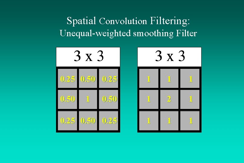
Spatial Convolution Filtering: Unequal-weighted smoothing Filter 0. 25 0. 50 0. 25 1 1 1 0. 50 1 2 1 0. 25 0. 50 0. 25 1 1

Spatial Convolution Filtering: Edge Enhancement For many remote sensing Earth science applications, the most valuable information that may be derived from an image is contained in the edges surrounding various objects of interest. Edge enhancement delineates these edges and makes the shapes and details comprising the image more conspicuous and perhaps easier to analyze. Edges may be enhanced using either linear or nonlinear edge enhancement techniques.

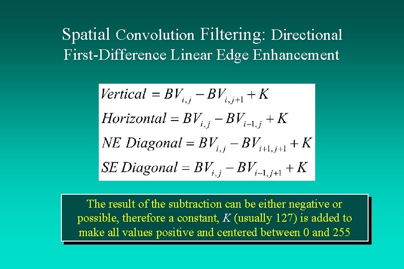
Spatial Convolution Filtering: Directional First-Difference Linear Edge Enhancement The result of the subtraction can be either negative or possible, therefore a constant, K (usually 127) is added to make all values positive and centered between 0 and 255

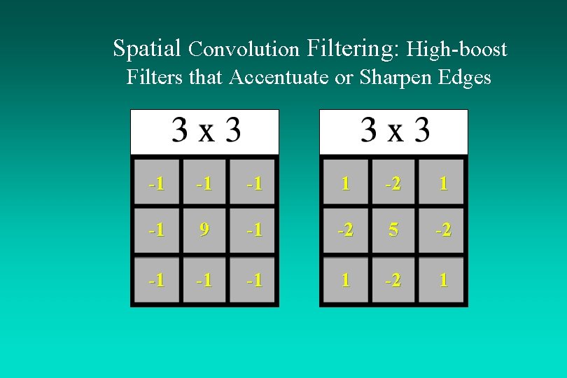
Spatial Convolution Filtering: High-boost Filters that Accentuate or Sharpen Edges -1 -1 -1 1 -2 1 -1 9 -1 -2 5 -2 -1 -1 -1 1 -2 1

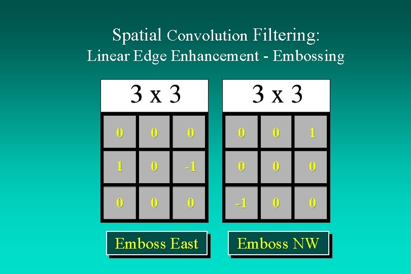
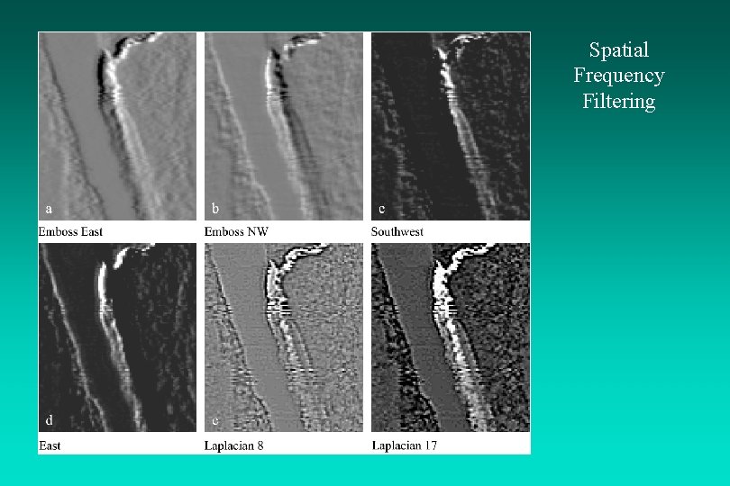
Spatial Convolution Filtering: Linear Edge Enhancement - Embossing 0 0 0 1 1 0 -1 0 0 Emboss East Emboss NW

Spatial Frequency Filtering

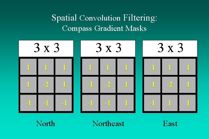
Spatial Convolution Filtering: Compass Gradient Masks 1 1 1 -1 1 -2 1 -1 -1 -1 1 1 Northeast East

Spatial Frequency Filtering

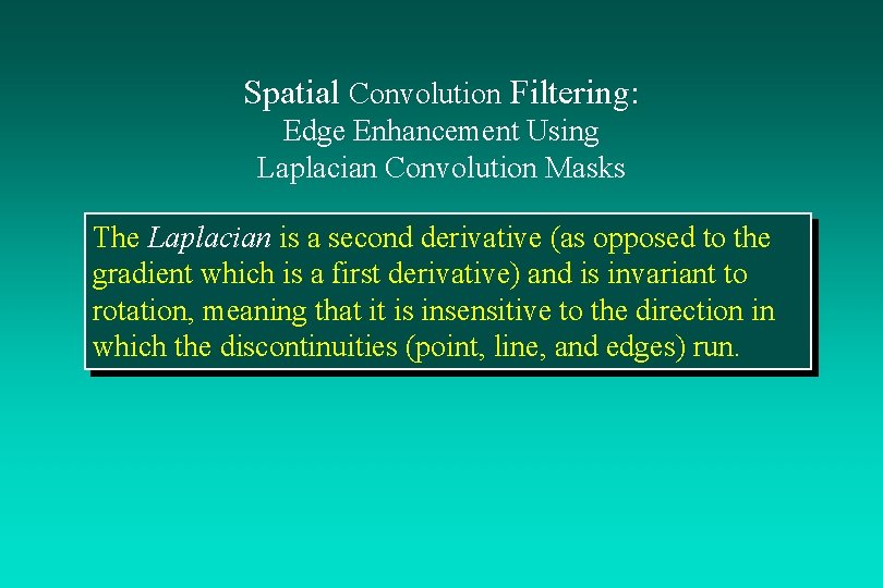
Spatial Convolution Filtering: Edge Enhancement Using Laplacian Convolution Masks The Laplacian is a second derivative (as opposed to the gradient which is a first derivative) and is invariant to rotation, meaning that it is insensitive to the direction in which the discontinuities (point, line, and edges) run.

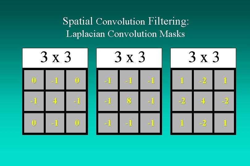
Spatial Convolution Filtering: Laplacian Convolution Masks 0 -1 -1 -1 1 -2 1 -1 4 -1 -1 8 -1 -2 4 -2 0 -1 -1 -1 1 -2 1

Spatial Frequency Filtering

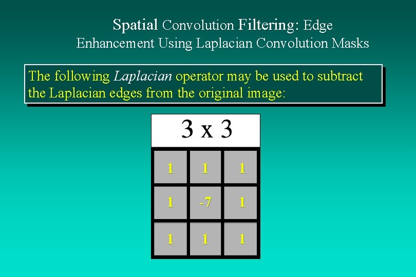
Spatial Convolution Filtering: Edge Enhancement Using Laplacian Convolution Masks The following Laplacian operator may be used to subtract the Laplacian edges from the original image: 1 1 -7 1 1

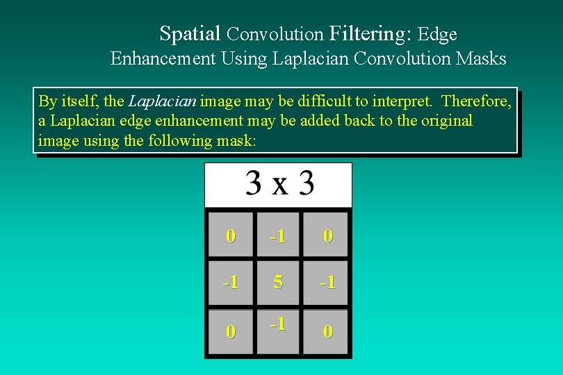
Spatial Convolution Filtering: Edge Enhancement Using Laplacian Convolution Masks By itself, the Laplacian image may be difficult to interpret. Therefore, a Laplacian edge enhancement may be added back to the original image using the following mask: 0 -1 5 -1 0

Spatial Frequency Filtering

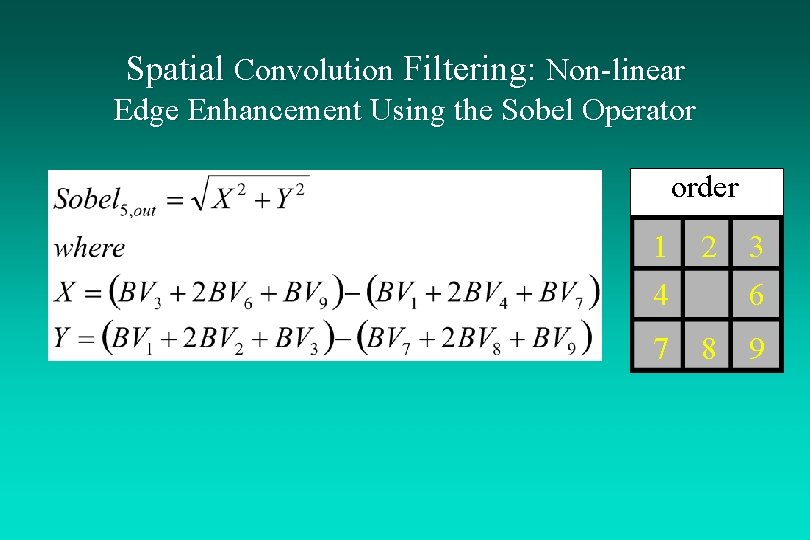
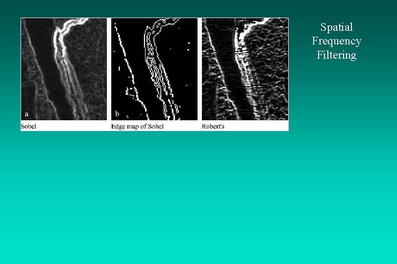
Spatial Convolution Filtering: Non-linear Edge Enhancement Using the Sobel Operator order 1 4 2 3 6 7 8 9

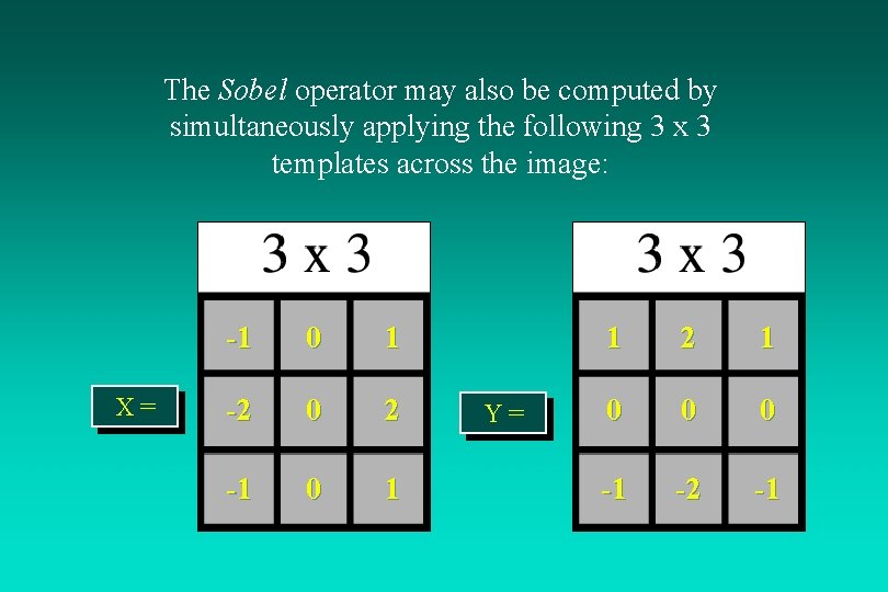
The Sobel operator may also be computed by simultaneously applying the following 3 x 3 templates across the image: X= -1 0 1 -2 0 2 -1 0 1 Y= 1 2 1 0 0 0 -1 -2 -1

Spatial Frequency Filtering

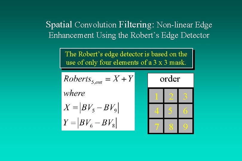
Spatial Convolution Filtering: Non-linear Edge Enhancement Using the Robert’s Edge Detector The Robert’s edge detector is based on the use of only four elements of a 3 x 3 mask. order 1 2 4 5 3 6 7 9 8

Spatial Frequency Filtering

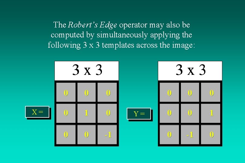
The Robert’s Edge operator may also be computed by simultaneously applying the following 3 x 3 templates across the image: X= 0 0 1 0 0 0 -1 Y= 0 0 0 1 0 -1 0

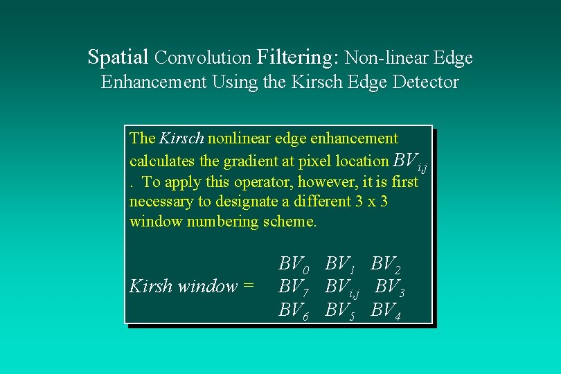
Spatial Convolution Filtering: Non-linear Edge Enhancement Using the Kirsch Edge Detector The Kirsch nonlinear edge enhancement calculates the gradient at pixel location BVi, j. To apply this operator, however, it is first necessary to designate a different 3 x 3 window numbering scheme. Kirsh window = BV 0 BV 7 BV 6 BV 1 BVi, j BV 5 BV 2 BV 3 BV 4

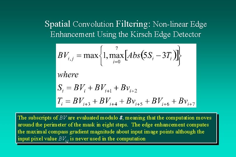
Spatial Convolution Filtering: Non-linear Edge Enhancement Using the Kirsch Edge Detector The subscripts of BV are evaluated modulo 8, meaning that the computation moves around the perimeter of the mask in eight steps. The edge enhancement computes the maximal compass gradient magnitude about input image points although the input pixel value BVi, j is never used in the computation