Spatial filtering for image sharpening Background Applications To

Spatial filtering for image sharpening Background: Applications: To highlight fine detail in an image or to enhance blurred detail Electronic printing, medical imaging, industrial inspection, autonomous target detection (smart weapons). . . Foundation: § Blurring/smoothing is performed by spatial averaging (equivalent to integration) § Sharpening is performed by noting only the gray level changes in the image that is the differentiation 11/1/2020 COMSATS Institute of Information Technology, Lahore Digital Image Processing CSC 331 1

Spatial filtering for image sharpening Operation of Image Differentiation § Enhance edges and discontinuities § De-emphasize areas with slowly varying gray-level values Mathematical Basis of Filtering for Image Sharpening § Implementation by mask filtering § First-order and second-order derivatives 11/1/2020 COMSATS Institute of Information Technology, Lahore Digital Image Processing CSC 331 2

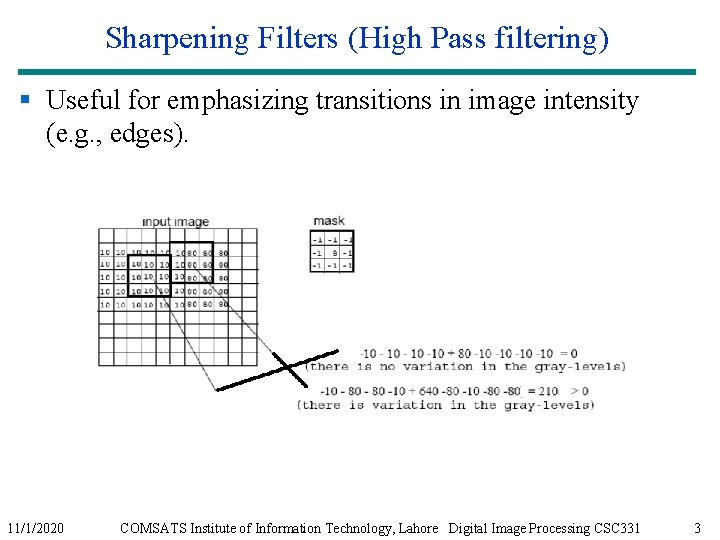
Sharpening Filters (High Pass filtering) § Useful for emphasizing transitions in image intensity (e. g. , edges). 11/1/2020 COMSATS Institute of Information Technology, Lahore Digital Image Processing CSC 331 3

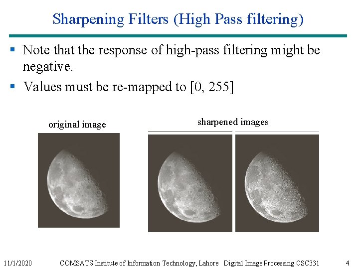
Sharpening Filters (High Pass filtering) § Note that the response of high-pass filtering might be negative. § Values must be re-mapped to [0, 255] original image 11/1/2020 sharpened images COMSATS Institute of Information Technology, Lahore Digital Image Processing CSC 331 4

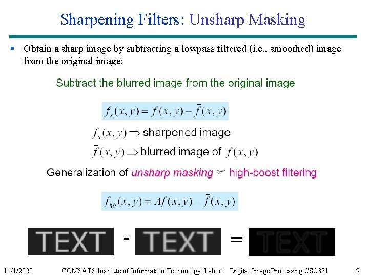
Sharpening Filters: Unsharp Masking § Obtain a sharp image by subtracting a lowpass filtered (i. e. , smoothed) image from the original image: 11/1/2020 = COMSATS Institute of Information Technology, Lahore Digital Image Processing CSC 331 5

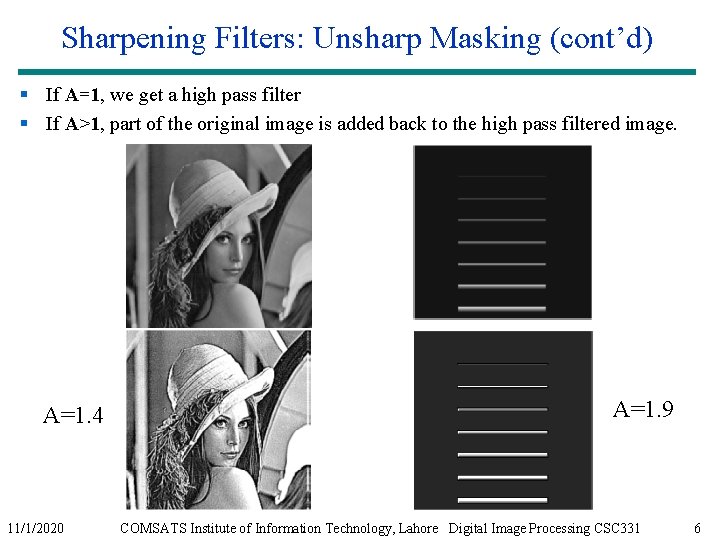
Sharpening Filters: Unsharp Masking (cont’d) § If A=1, we get a high pass filter § If A>1, part of the original image is added back to the high pass filtered image. A=1. 4 11/1/2020 A=1. 9 COMSATS Institute of Information Technology, Lahore Digital Image Processing CSC 331 6

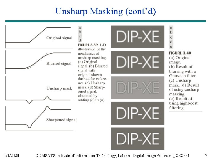
Unsharp Masking (cont’d) 11/1/2020 COMSATS Institute of Information Technology, Lahore Digital Image Processing CSC 331 7

Image sharpening (High-Pass Filters) § Spatial filters whose effect on the output image is equivalent to preserving or emphasizing its highfrequency components (e. g. , fine details, points, lines, and edges), i. e. to highlight transitions in intensity within the image. § Linear HPFs can be implemented using 2 D masks with positive and negative weights / coefficients, (Laplacian, a simple, isotropic (i. e. , rotation invariant) second-order derivative) 11/1/2020 COMSATS Institute of Information Technology, Lahore Digital Image Processing CSC 331 8

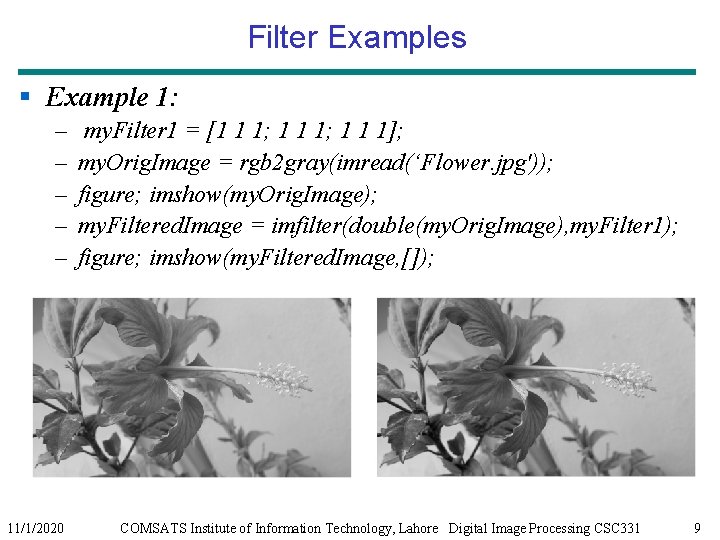
Filter Examples § Example 1: – – – 11/1/2020 my. Filter 1 = [1 1 1; 1 1 1]; my. Orig. Image = rgb 2 gray(imread(‘Flower. jpg')); figure; imshow(my. Orig. Image); my. Filtered. Image = imfilter(double(my. Orig. Image), my. Filter 1); figure; imshow(my. Filtered. Image, []); COMSATS Institute of Information Technology, Lahore Digital Image Processing CSC 331 9

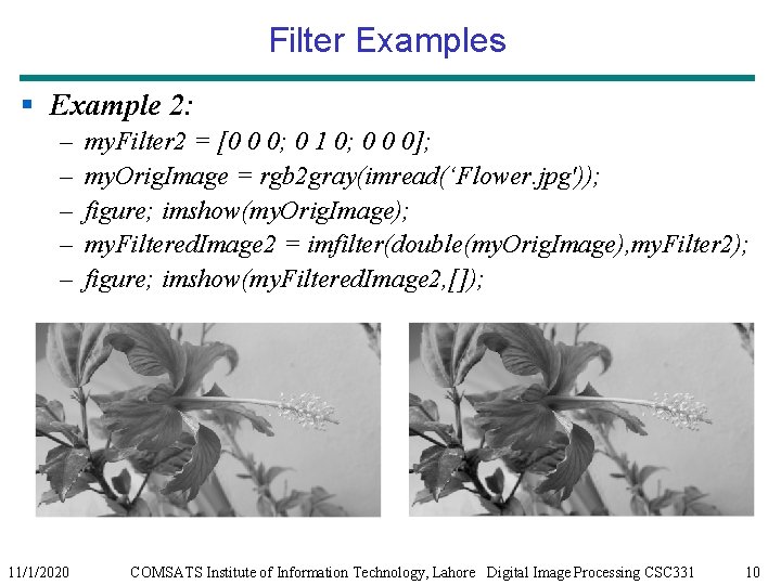
Filter Examples § Example 2: – – – 11/1/2020 my. Filter 2 = [0 0 0; 0 1 0; 0 0 0]; my. Orig. Image = rgb 2 gray(imread(‘Flower. jpg')); figure; imshow(my. Orig. Image); my. Filtered. Image 2 = imfilter(double(my. Orig. Image), my. Filter 2); figure; imshow(my. Filtered. Image 2, []); COMSATS Institute of Information Technology, Lahore Digital Image Processing CSC 331 10

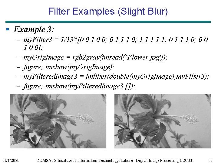
Filter Examples (Slight Blur) § Example 3: – my. Filter 3 = 1/13*[0 0 1 0 0; 0 1 1 1 0; 1 1 1; 0 1 1 1 0; 0 0 1 0 0]; – my. Orig. Image = rgb 2 gray(imread(‘Flower. jpg')); – figure; imshow(my. Orig. Image); – my. Filtered. Image 3 = imfilter(double(my. Orig. Image), my. Filter 3); – figure; imshow(my. Filtered. Image 3, []); 11/1/2020 COMSATS Institute of Information Technology, Lahore Digital Image Processing CSC 331 11

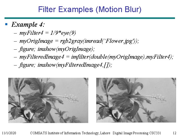
Filter Examples (Motion Blur) § Example 4: – – – 11/1/2020 my. Filter 4 = 1/9*eye(9) my. Orig. Image = rgb 2 gray(imread(‘Flower. jpg')); figure; imshow(my. Orig. Image); my. Filtered. Image 4 = imfilter(double(my. Orig. Image), my. Filter 4); figure; imshow(my. Filtered. Image 4, []); COMSATS Institute of Information Technology, Lahore Digital Image Processing CSC 331 12

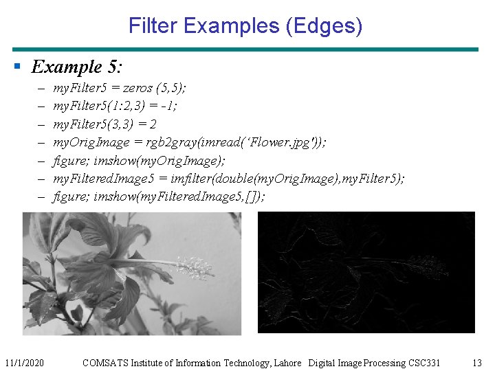
Filter Examples (Edges) § Example 5: – – – – 11/1/2020 my. Filter 5 = zeros (5, 5); my. Filter 5(1: 2, 3) = -1; my. Filter 5(3, 3) = 2 my. Orig. Image = rgb 2 gray(imread(‘Flower. jpg')); figure; imshow(my. Orig. Image); my. Filtered. Image 5 = imfilter(double(my. Orig. Image), my. Filter 5); figure; imshow(my. Filtered. Image 5, []); COMSATS Institute of Information Technology, Lahore Digital Image Processing CSC 331 13

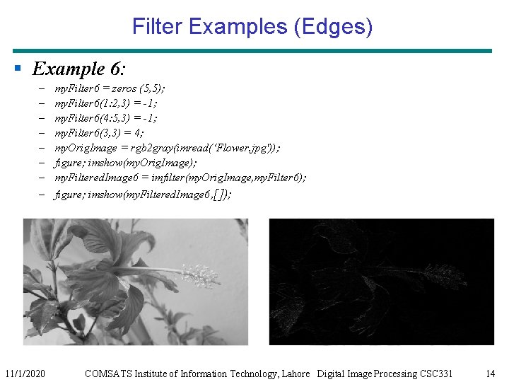
Filter Examples (Edges) § Example 6: – – – – 11/1/2020 my. Filter 6 = zeros (5, 5); my. Filter 6(1: 2, 3) = -1; my. Filter 6(4: 5, 3) = -1; my. Filter 6(3, 3) = 4; my. Orig. Image = rgb 2 gray(imread(‘Flower. jpg')); figure; imshow(my. Orig. Image); my. Filtered. Image 6 = imfilter(my. Orig. Image, my. Filter 6); figure; imshow(my. Filtered. Image 6, []); COMSATS Institute of Information Technology, Lahore Digital Image Processing CSC 331 14

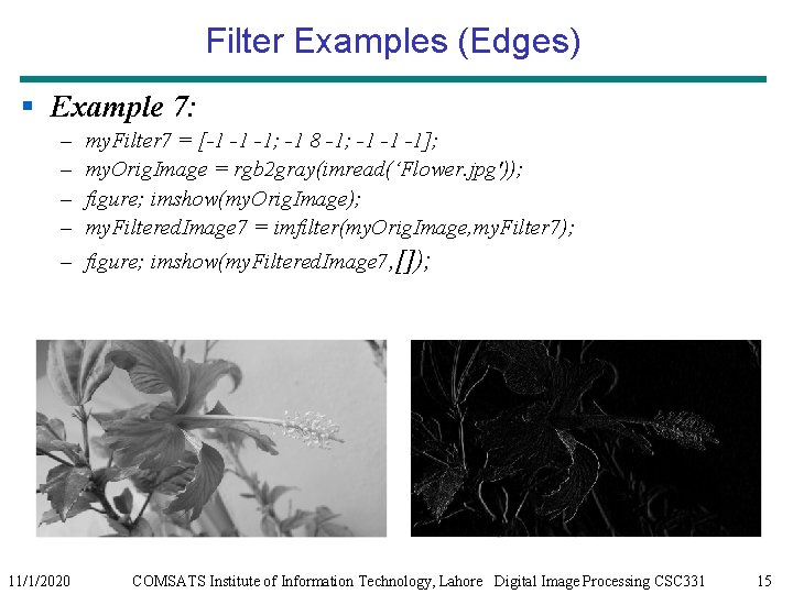
Filter Examples (Edges) § Example 7: – – my. Filter 7 = [-1 -1 -1; -1 8 -1; -1 -1 -1]; my. Orig. Image = rgb 2 gray(imread(‘Flower. jpg')); figure; imshow(my. Orig. Image); my. Filtered. Image 7 = imfilter(my. Orig. Image, my. Filter 7); – figure; imshow(my. Filtered. Image 7, []); 11/1/2020 COMSATS Institute of Information Technology, Lahore Digital Image Processing CSC 331 15

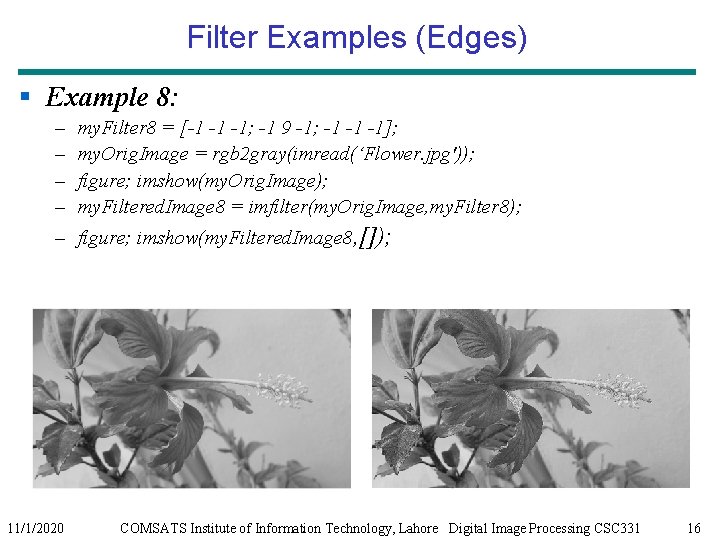
Filter Examples (Edges) § Example 8: – – my. Filter 8 = [-1 -1 -1; -1 9 -1; -1 -1 -1]; my. Orig. Image = rgb 2 gray(imread(‘Flower. jpg')); figure; imshow(my. Orig. Image); my. Filtered. Image 8 = imfilter(my. Orig. Image, my. Filter 8); – figure; imshow(my. Filtered. Image 8, []); 11/1/2020 COMSATS Institute of Information Technology, Lahore Digital Image Processing CSC 331 16

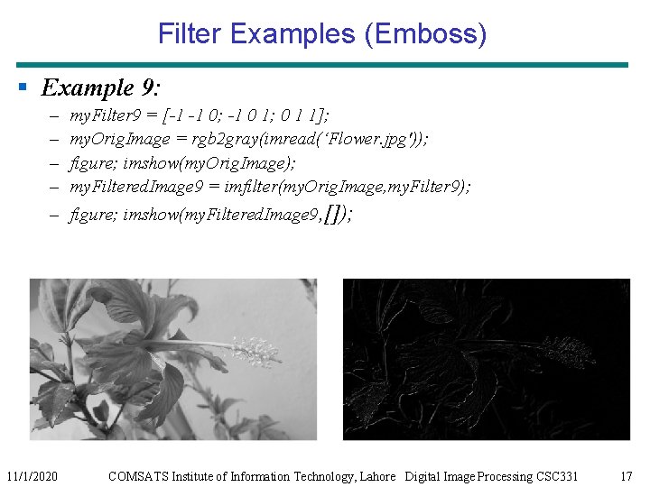
Filter Examples (Emboss) § Example 9: – – my. Filter 9 = [-1 -1 0; -1 0 1; 0 1 1]; my. Orig. Image = rgb 2 gray(imread(‘Flower. jpg')); figure; imshow(my. Orig. Image); my. Filtered. Image 9 = imfilter(my. Orig. Image, my. Filter 9); – figure; imshow(my. Filtered. Image 9, []); 11/1/2020 COMSATS Institute of Information Technology, Lahore Digital Image Processing CSC 331 17

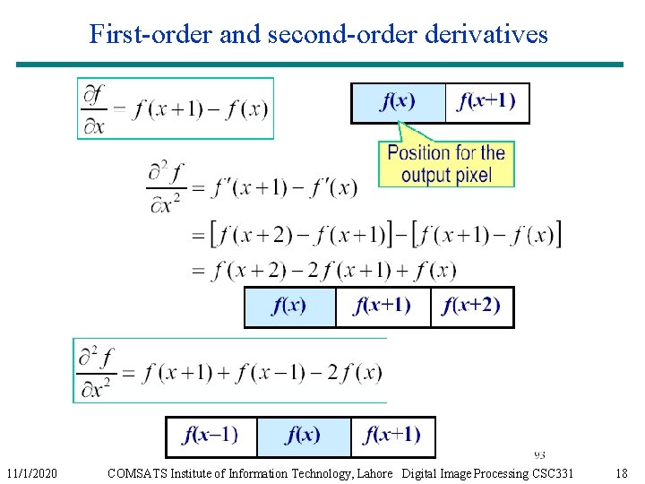
First-order and second-order derivatives 11/1/2020 COMSATS Institute of Information Technology, Lahore Digital Image Processing CSC 331 18

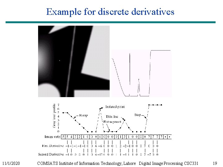
Example for discrete derivatives 11/1/2020 COMSATS Institute of Information Technology, Lahore Digital Image Processing CSC 331 19

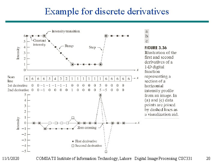
Example for discrete derivatives 11/1/2020 COMSATS Institute of Information Technology, Lahore Digital Image Processing CSC 331 20

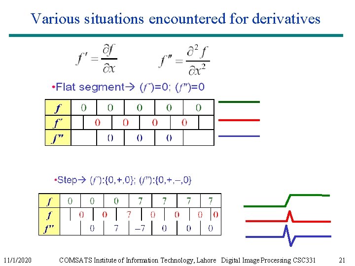
Various situations encountered for derivatives 11/1/2020 COMSATS Institute of Information Technology, Lahore Digital Image Processing CSC 331 21

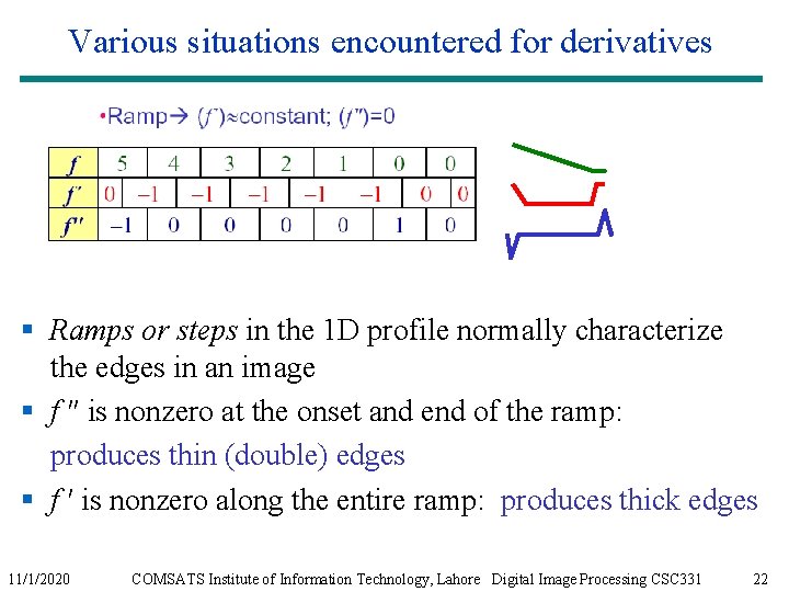
Various situations encountered for derivatives § Ramps or steps in the 1 D profile normally characterize the edges in an image § f ″ is nonzero at the onset and end of the ramp: produces thin (double) edges § f ′ is nonzero along the entire ramp: produces thick edges 11/1/2020 COMSATS Institute of Information Technology, Lahore Digital Image Processing CSC 331 22

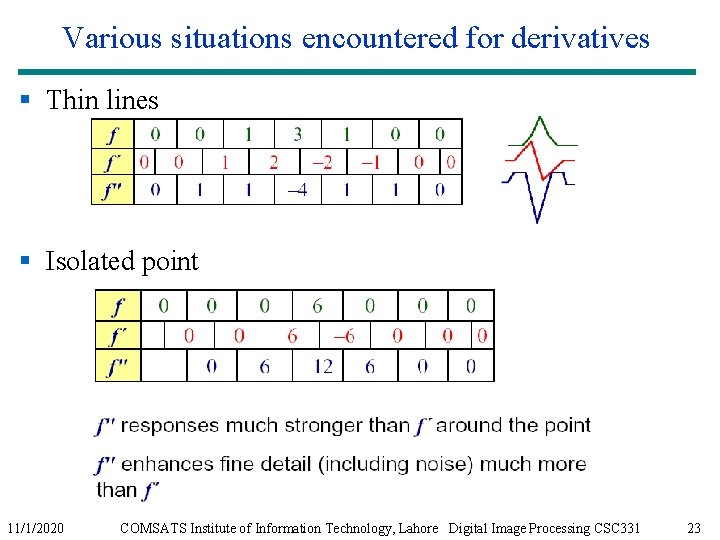
Various situations encountered for derivatives § Thin lines § Isolated point 11/1/2020 COMSATS Institute of Information Technology, Lahore Digital Image Processing CSC 331 23

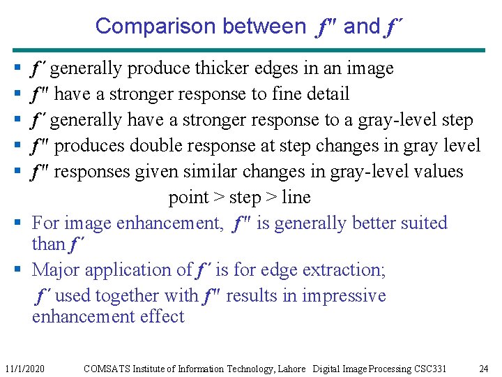
Comparison between f" and f´ § § § f´ generally produce thicker edges in an image f" have a stronger response to fine detail f´ generally have a stronger response to a gray-level step f" produces double response at step changes in gray level f" responses given similar changes in gray-level values point > step > line § For image enhancement, f" is generally better suited than f´ § Major application of f´ is for edge extraction; f´ used together with f" results in impressive enhancement effect 11/1/2020 COMSATS Institute of Information Technology, Lahore Digital Image Processing CSC 331 24

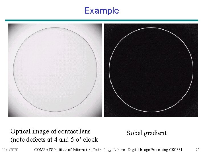
Example Optical image of contact lens (note defects at 4 and 5 o’ clock 11/1/2020 Sobel gradient COMSATS Institute of Information Technology, Lahore Digital Image Processing CSC 331 25