Spatial Filtering CS 474674 Prof Bebis Sections 3

Spatial Filtering CS 474/674 - Prof. Bebis Sections 3. 4, 3. 5, 3. 6, 3. 7, 3. 8

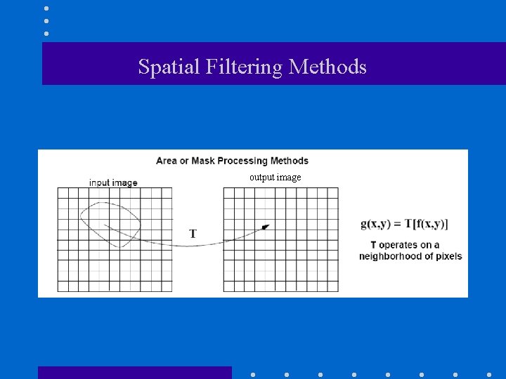
Spatial Filtering Methods output image

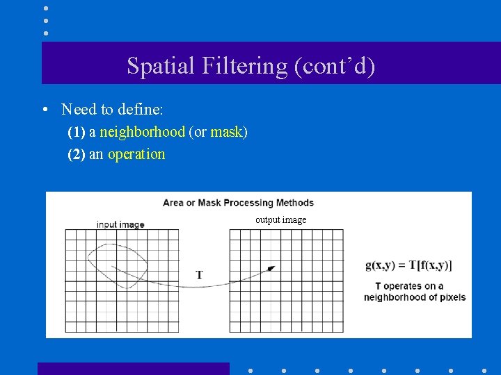
Spatial Filtering (cont’d) • Need to define: (1) a neighborhood (or mask) (2) an operation output image

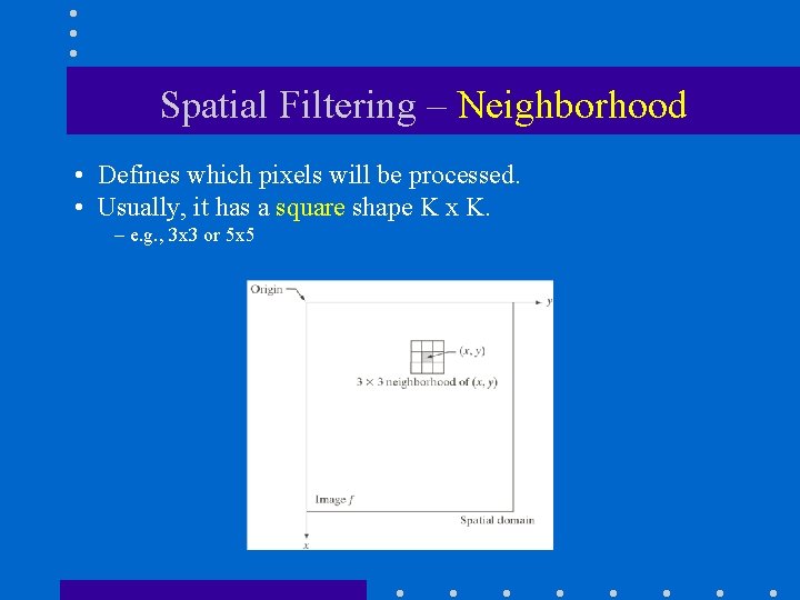
Spatial Filtering – Neighborhood • Defines which pixels will be processed. • Usually, it has a square shape K x K. – e. g. , 3 x 3 or 5 x 5

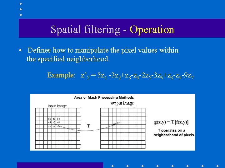
Spatial filtering - Operation • Defines how to manipulate the pixel values within the specified neighborhood. Example: z’ 5 = 5 z 1 -3 z 2+z 3 -z 4 -2 z 5 -3 z 6+z 8 -z 9 -9 z 7 output image

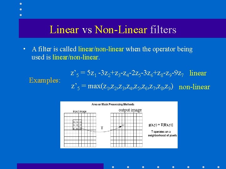
Linear vs Non-Linear filters • A filter is called linear/non-linear when the operator being used is linear/non-linear. Examples: z’ 5 = 5 z 1 -3 z 2+z 3 -z 4 -2 z 5 -3 z 6+z 8 -z 9 -9 z 7 linear z’ 5 = max(z 1, z 2, z 3, z 4, z 5, z 6, z 7, z 8, z 9) non-linear output image

Linear Operators • Two common linear operators are: – Correlation – Convolution • The output is a linear combination of the inputs.

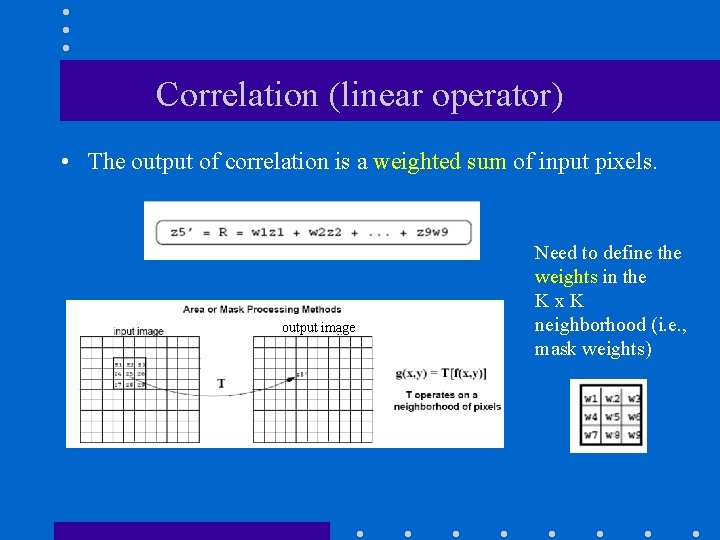
Correlation (linear operator) • The output of correlation is a weighted sum of input pixels. output image Need to define the weights in the K x K neighborhood (i. e. , mask weights)

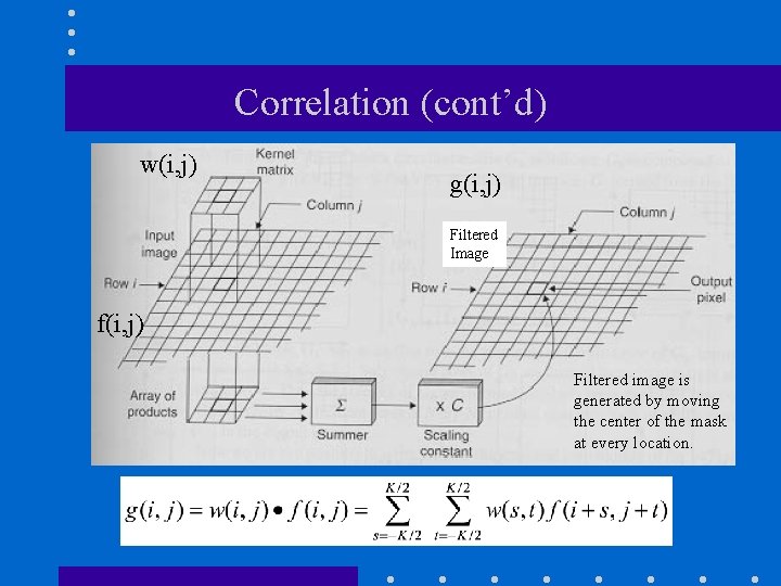
Correlation (cont’d) w(i, j) g(i, j) Filtered Image f(i, j) Filtered image is generated by moving the center of the mask at every location.

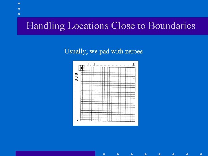
Handling Locations Close to Boundaries Usually, we pad with zeroes 0 0 0 ………………………. 0

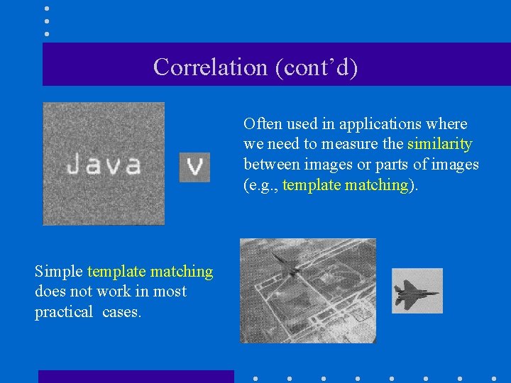
Correlation (cont’d) Often used in applications where we need to measure the similarity between images or parts of images (e. g. , template matching). Simple template matching does not work in most practical cases.

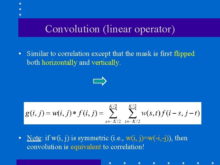
Convolution (linear operator) • Similar to correlation except that the mask is first flipped both horizontally and vertically. • Note: if w(i, j) is symmetric (i. e. , w(i, j)=w(-i, -j)), then convolution is equivalent to correlation!

Example Correlation: Convolution:

Filter Categories • We will focus on two types of filters: – Smoothing (low-pass) filters – Sharpening (high-pass) filters

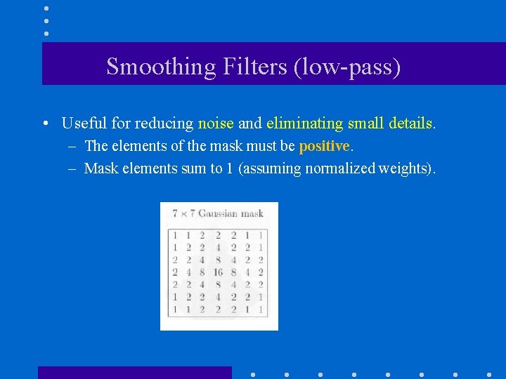
Smoothing Filters (low-pass) • Useful for reducing noise and eliminating small details. – The elements of the mask must be positive. – Mask elements sum to 1 (assuming normalized weights).

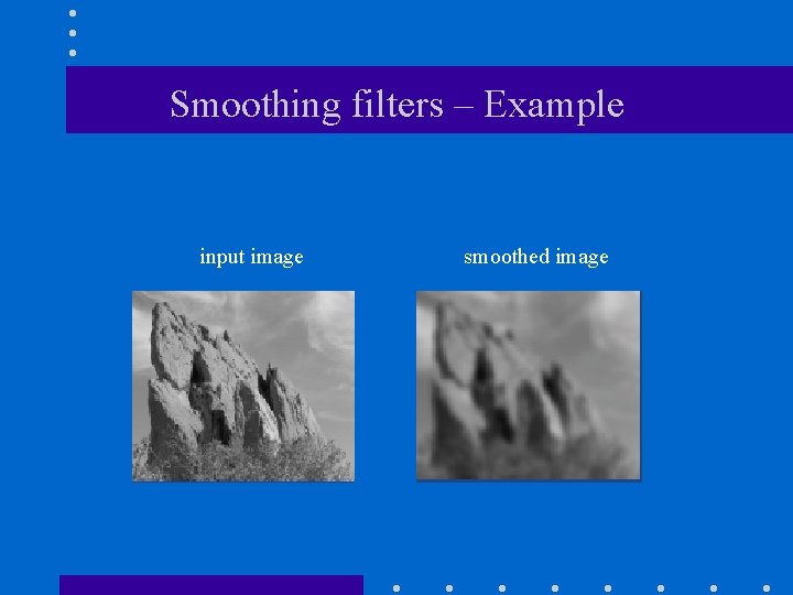
Smoothing filters – Example input image smoothed image

Sharpening Filters (high-pass) • Useful for highlighting fine details. – The elements of the mask contain both positive and negative weights. – Mask elements sum to 0.

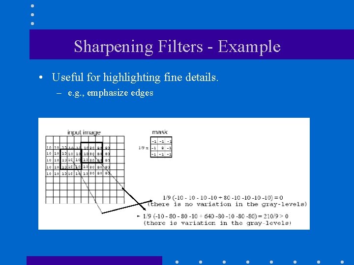
Sharpening Filters - Example • Useful for highlighting fine details. – e. g. , emphasize edges

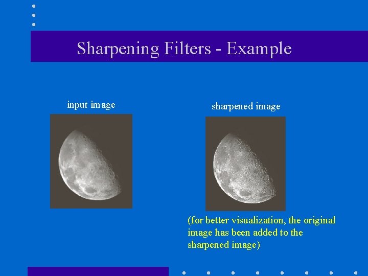
Sharpening Filters - Example input image sharpened image (for better visualization, the original image has been added to the sharpened image)

Common Smoothing Filters • Averaging • Gaussian • Median filtering (non-linear)

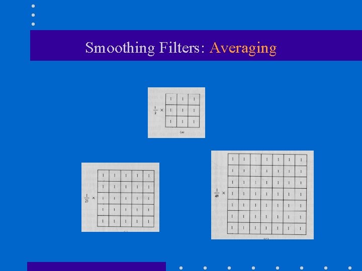
Smoothing Filters: Averaging

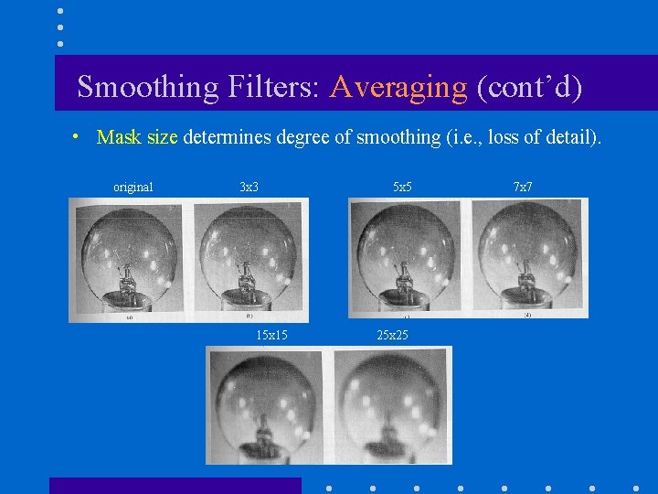
Smoothing Filters: Averaging (cont’d) • Mask size determines degree of smoothing (i. e. , loss of detail). original 3 x 3 15 x 15 5 x 5 25 x 25 7 x 7

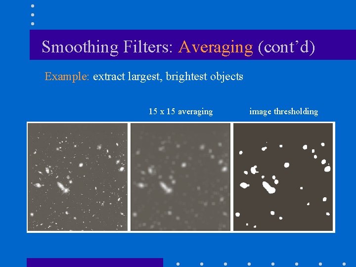
Smoothing Filters: Averaging (cont’d) Example: extract largest, brightest objects 15 x 15 averaging image thresholding

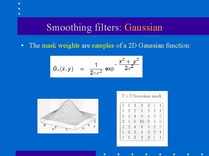
Smoothing filters: Gaussian • The mask weights are samples of a 2 D Gaussian function:

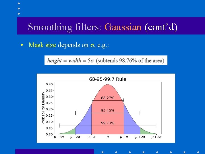
Smoothing filters: Gaussian (cont’d) • Mask size depends on σ, e. g. :

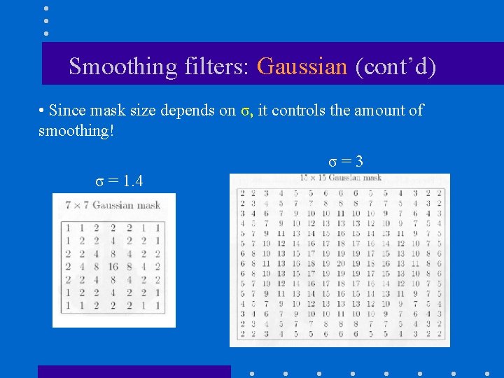
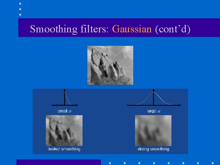
Smoothing filters: Gaussian (cont’d) • Since mask size depends on σ, it controls the amount of smoothing! σ = 3 σ = 1. 4

Smoothing filters: Gaussian (cont’d)

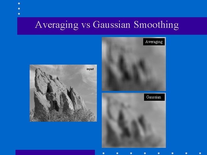
Averaging vs Gaussian Smoothing Averaging Gaussian

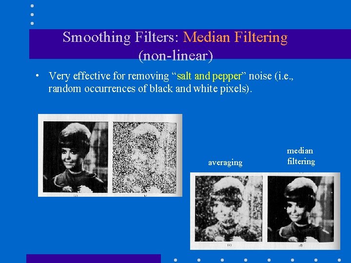
Smoothing Filters: Median Filtering (non-linear) • Very effective for removing “salt and pepper” noise (i. e. , random occurrences of black and white pixels). averaging median filtering

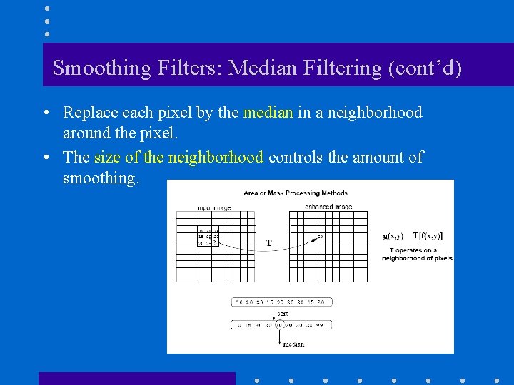
Smoothing Filters: Median Filtering (cont’d) • Replace each pixel by the median in a neighborhood around the pixel. • The size of the neighborhood controls the amount of smoothing.

Common Sharpening Filters • • Unsharp masking High Boost filter Gradient (1 st derivative) Laplacian (2 nd derivative)

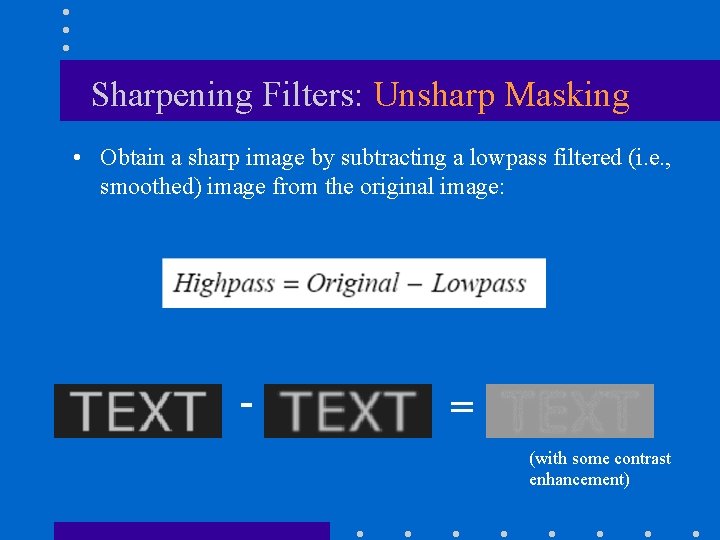
Sharpening Filters: Unsharp Masking • Obtain a sharp image by subtracting a lowpass filtered (i. e. , smoothed) image from the original image: - = (with some contrast enhancement)

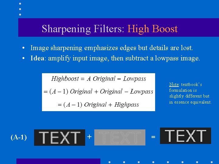
Sharpening Filters: High Boost • Image sharpening emphasizes edges but details are lost. • Idea: amplify input image, then subtract a lowpass image. Note: textbook’s formulation is slightly different but in essence equivalent. (A-1) + =

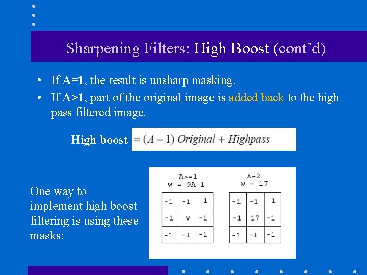
Sharpening Filters: High Boost (cont’d) • If A=1, the result is unsharp masking. • If A>1, part of the original image is added back to the high pass filtered image. High boost One way to implement high boost filtering is using these masks:

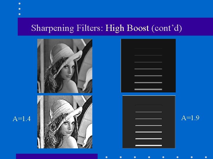
Sharpening Filters: High Boost (cont’d) A=1. 4 A=1. 9

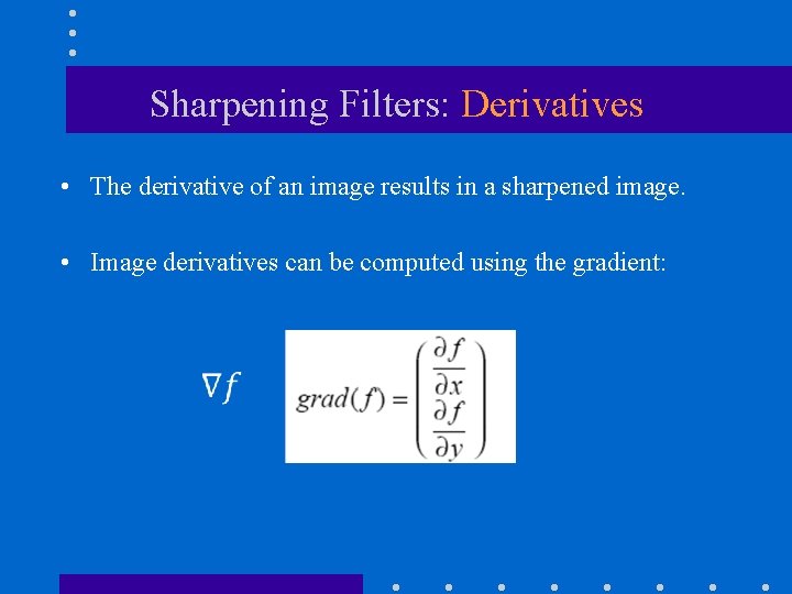
Sharpening Filters: Derivatives • The derivative of an image results in a sharpened image. • Image derivatives can be computed using the gradient:

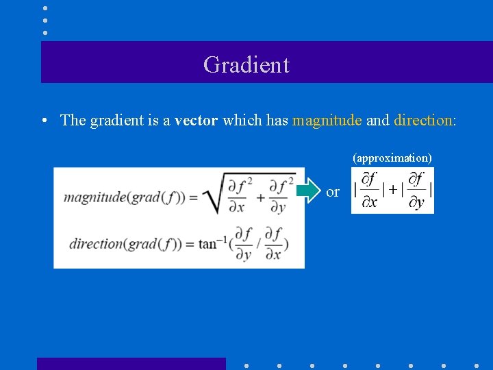
Gradient • The gradient is a vector which has magnitude and direction: (approximation) or

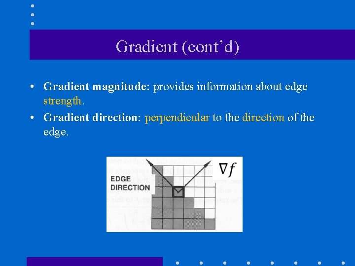
Gradient (cont’d) • Gradient magnitude: provides information about edge strength. • Gradient direction: perpendicular to the direction of the edge.

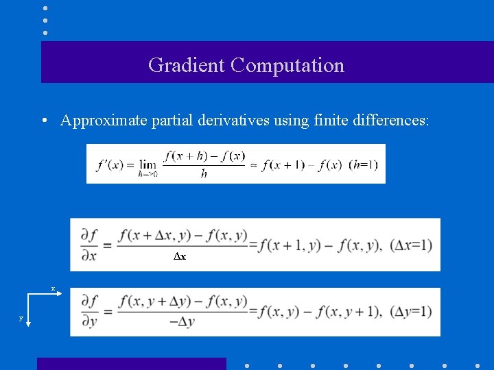
Gradient Computation • Approximate partial derivatives using finite differences: Δx x y

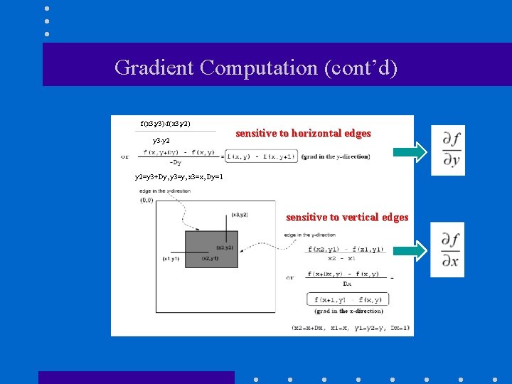
Gradient Computation (cont’d) f(x 3, y 3)-f(x 3, y 2) y 3 -y 2 sensitive to horizontal edges y 2=y 3+Dy, y 3=y, x 3=x, Dy=1 sensitive to vertical edges

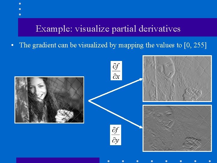
Example: visualize partial derivatives • The gradient can be visualized by mapping the values to [0, 255]

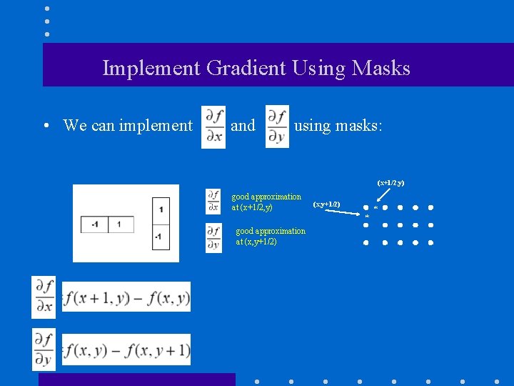
Implement Gradient Using Masks • We can implement and using masks: (x+1/2, y) good approximation at (x+1/2, y) (x, y+1/2) * * good approximation at (x, y+1/2)

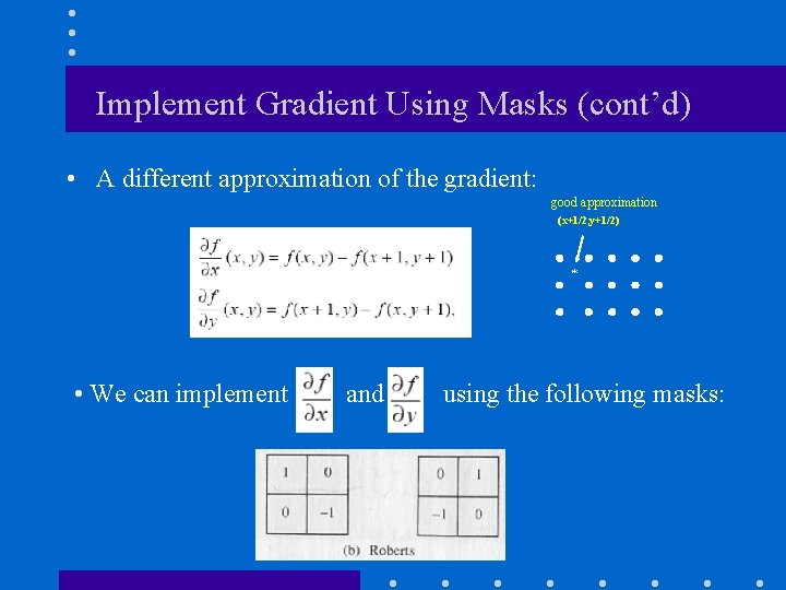
Implement Gradient Using Masks (cont’d) • A different approximation of the gradient: good approximation (x+1/2, y+1/2) * • We can implement and using the following masks:

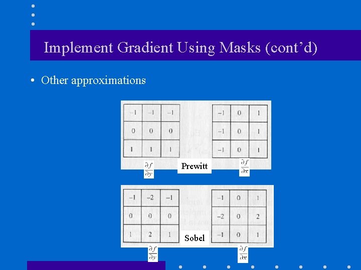
Implement Gradient Using Masks (cont’d) • Other approximations Prewitt Sobel

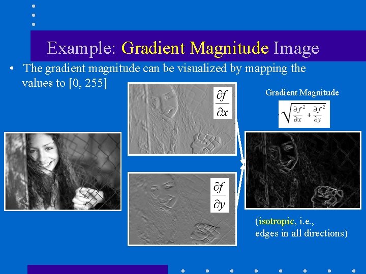
Example: Gradient Magnitude Image • The gradient magnitude can be visualized by mapping the values to [0, 255] Gradient Magnitude (isotropic, i. e. , edges in all directions)

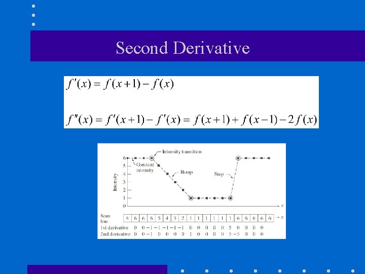
Second Derivative

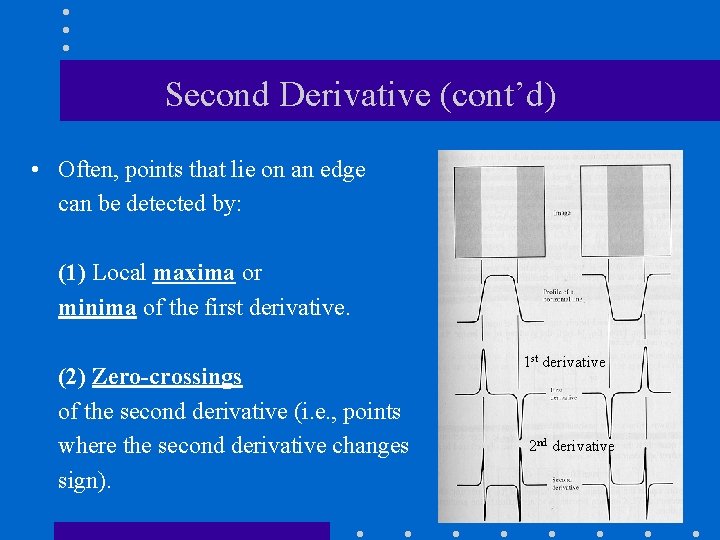
Second Derivative (cont’d) • Often, points that lie on an edge can be detected by: (1) Local maxima or minima of the first derivative. (2) Zero-crossings of the second derivative (i. e. , points where the second derivative changes sign). 1 st derivative 2 nd derivative

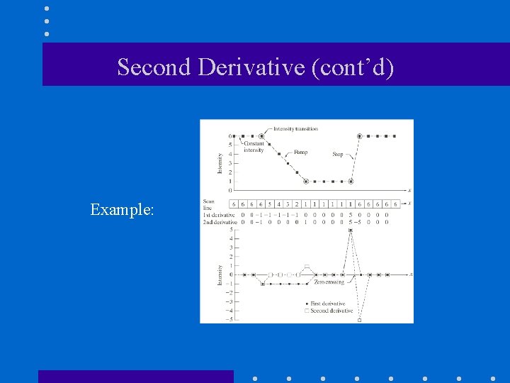
Second Derivative (cont’d) Example:

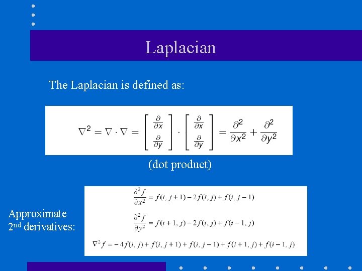
Laplacian The Laplacian is defined as: (dot product) Approximate 2 nd derivatives:

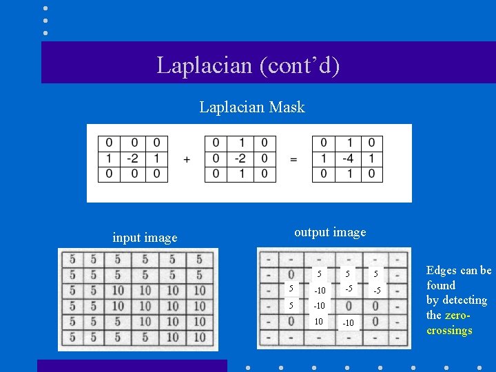
Laplacian (cont’d) Laplacian Mask output image input image 5 5 -10 -5 -5 5 -10 10 -10 Edges can be found by detecting the zerocrossings

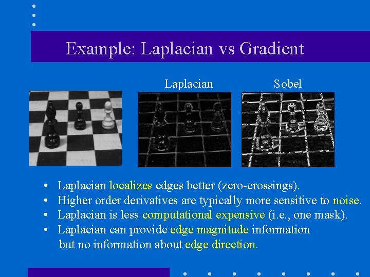
Example: Laplacian vs Gradient Laplacian Sobel • Laplacian localizes edges better (zero-crossings). • Higher order derivatives are typically more sensitive to noise. • Laplacian is less computational expensive (i. e. , one mask). • Laplacian can provide edge magnitude information but no information about edge direction.

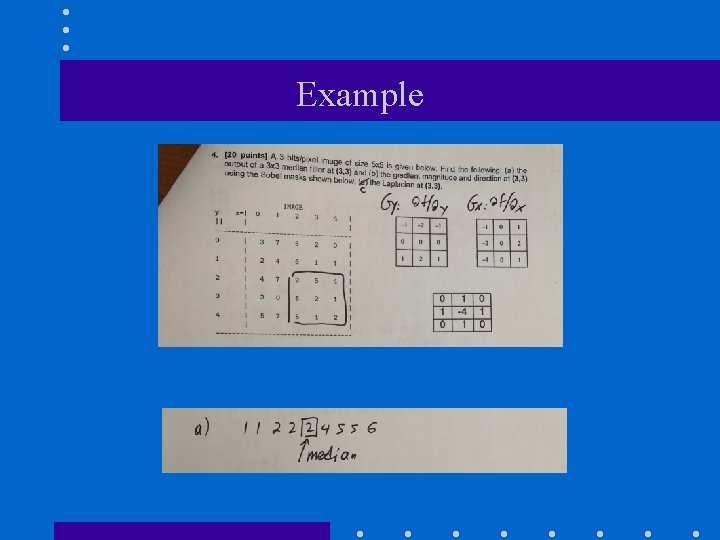
Example

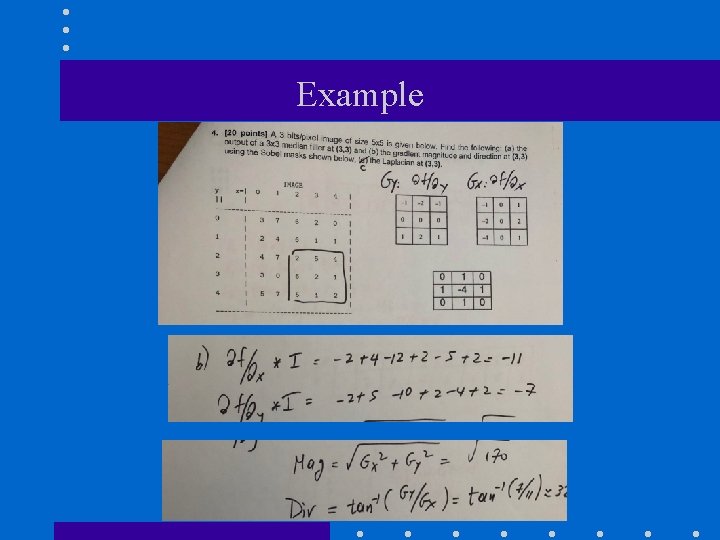
Example

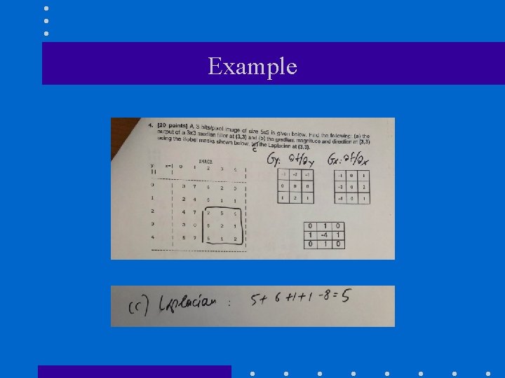
Example

Quiz #3 • When: Monday (Oct 12 th) at 2 pm • What: Spatial Transformations • Duration – 10 minutes for answering questions – 5 minutes for uploading your answers on Canvas • Suggested Apps – Genius Scan https: //thegrizzlylabs. com/genius-scan/ – Canvas Student https: //apps. apple. com/us/app/canvas-student/id 480883488