Spatial Fields in GIS and Hydrology David G

Spatial Fields in GIS and Hydrology David G. Tarboton dtarb@cc. usu. edu http: //www. engineering. usu. edu/dtarb

Learning Objectives n n The concepts of spatial fields as a way to represent geographical information Raster and vector representations of spatial fields Raster based watershed delineation from digital elevation models Reading – Arc. Hydro Chapter 4

Two fundamental ways of representing geography are discrete objects and fields. The discrete object view represents the real world as objects with well defined boundaries in empty space. (x 1, y 1) Points Lines Polygons The field view represents the real world as a finite number of variables, each one defined at each possible position. f(x, y) y Continuous surface x

Raster and Vector Data Raster data are described by a cell grid, one value per cell Vector Raster Point Line Zone of cells Polygon

Raster and Vector are two methods of representing geographic data in GIS • Both represent different ways to encode and generalize geographic phenomena • Both can be used to code both fields and discrete objects • In practice a strong association between raster and fields and vector and discrete objects

Vector and Raster Representation of Spatial Fields Vector Raster

Numerical representation of a spatial surface (field) Grid TIN Contour and flowline

Six approximate representations of a field used in GIS Regularly spaced sample points Irregularly shaped polygons Irregularly spaced sample points Triangulated Irregular Network (TIN) Rectangular Cells Polylines/Contours from Longley, P. A. , M. F. Goodchild, D. J. Maguire and D. W. Rind, (2001), Geographic Information Systems and Science, Wiley, 454 p.

A grid defines geographic space as a matrix of identically-sized square cells. Each cell holds a numeric value that measures a geographic attribute (like elevation) for that unit of space.

The grid data structure • Grid size is defined by extent, spacing and no data value information – Number of rows, number of column – Cell sizes (X and Y) – Top, left , bottom and right coordinates • Grid values – Real (floating decimal point) – Integer (may have associated attribute table)

Definition of a Grid Cell size Number of rows NODATA cell (X, Y) Number of Columns

Points as Cells

Line as a Sequence of Cells

Polygon as a Zone of Cells

NODATA Cells

Cell Networks

Grid Zones

Floating Point Grids Continuous data surfaces using floating point or decimal numbers

Value attribute table for categorical (integer) grid data Attributes of grid zones

Raster Sampling from Michael F. Goodchild. (1997) Rasters, NCGIA Core Curriculum in GIScience, http: //www. ncgia. ucsb. edu/giscc/units/u 055. html, posted October 23, 1997

Scale issues in the interpretation of data The scale triplet a) Extent b) Spacing c) Support From: Blöschl, G. , (1996), Scale and Scaling in Hydrology, Habilitationsschrift, Weiner Mitteilungen Wasser Abwasser Gewasser, Wien, 346 p.

From: Blöschl, G. , (1996), Scale and Scaling in Hydrology, Habilitationsschrift, Weiner Mitteilungen Wasser Abwasser Gewasser, Wien, 346 p.

Raster Generalization Largest share rule Central point rule

Spatial Surfaces used in Hydrology Elevation Surface — the ground surface elevation at each point

Topographic Slope • Defined or represented by one of the following – Surface derivative z (dz/dx, dz/dy) – Vector with x and y components (Sx, Sy) – Vector with magnitude (slope) and direction (aspect) (S, )

Standard Slope Function a b c d g e h f i

Aspect – the steepest downslope direction

Example 30 a d g 80 69 60 b e h 74 67 52 c 63 f 145. 2 o 56 i 48

Hydrologic Slope - Direction of Steepest Descent 30 30 80 74 63 69 67 56 60 52 48 Slope: Arc. Hydro Page 70

Eight Direction Pour Point Model 32 64 1 16 8 128 4 2 ESRI Direction encoding Arc. Hydro Page 69

Limitation due to 8 grid directions. ?

The D Algorithm Tarboton, D. G. , (1997), "A New Method for the Determination of Flow Directions and Contributing Areas in Grid Digital Elevation Models, " Water Resources Research, 33(2): 309 -319. ) (http: //www. engineering. usu. edu/cee/faculty/dtarb/dinf. pdf)

The D Algorithm If 1 is not fit within the triangle the angle is chosen along the steepest edge or diagonal resulting in a slope and direction equivalent to D 8

D∞ Example 30 80 69 60 284. 9 o 74 eo 67 e 7 52 14. 9 o 63 56 e 8 48

DEM Based Watershed and Stream Network Delineation • Study Area in West Austin with a USGS 30 m DEM from a 1: 24, 000 scale map • Eight direction pour point model (flow direction and flow accumulation grids) • Stream network definition • Watershed delineation

Watershed Delineation by Hand Digitizing Watershed divide Drainage direction Arc. Hydro Page 57 Outlet

DEM Elevations 720 Contours 740 720 700 680

32 Flow Direction Grid 1 16 8 Arc. Hydro Page 71 64 128 4 2 2 2 4 4 8 1 2 4 8 4 128 1 2 4 8 2 1 4 4 4 1 1 1 2 16

Flow Direction Grid 32 64 128 16 8 1 4 2

Grid Network Arc. Hydro Page 71

Contributing Area Grid 1 1 1 1 4 3 3 1 1 12 1 1 2 16 1 1 1 3 6 25 2 1 1 4 3 1 1 1 12 2 1 3 16 6 25 2 1 2 Tau. DEM convention. The area draining each grid cell including the grid cell itself.

Flow Accumulation Grid. ESRI convention. Area draining in to a grid cell 0 0 3 0 0 0 0 2 11 1 2 5 0 0 0 0 2 0 0 0 3 2 2 0 1 0 0 11 0 0 0 1 15 0 0 2 5 24 1 15 24 1 Link to Grid calculator Arc. Hydro Page 72

Flow Accumulation > 5 Cell Threshold 0 0 0 3 2 2 0 0 0 11 0 0 1 15 0 0 2 5 24 1

Stream Network for 5 cell Threshold Drainage Area 0 0 3 0 0 0 2 0 0 0 11 1 0 2 1 0 15 5 24 1

Streams with 200 cell Threshold (>18 hectares or 13. 5 acres drainage area)

Watershed Outlet

Watershed Draining to This Outlet

Watershed and Drainage Paths Delineated from 30 m DEM Automated method is more consistent than hand delineation

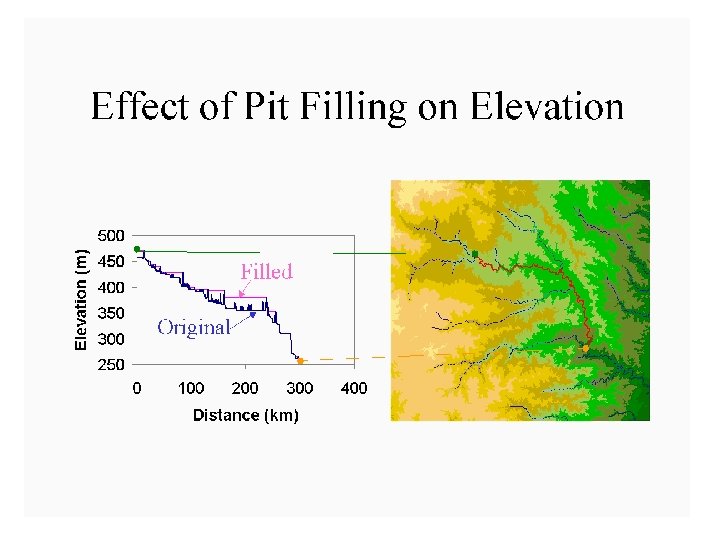
Filling in the Pits • DEM creation results in artificial pits in the landscape • A pit is a set of one or more cells which has no downstream cells around it • Unless these pits are filled they become sinks and isolate portions of the watershed • Pit filling is first thing done with a DEM

“Burning In” the Streams Take a mapped stream network and a DEM Make a grid of the streams Raise the off-stream DEM cells by an arbitrary elevation increment Produces "burned in" DEM streams = mapped streams + =

AGREE Elevation Grid Modification Methodology

Stream Segments 0 0 3 0 0 0 2 0 0 0 11 1 0 2 1 0 15 5 24 1

Stream Links in a Cell Network 1 1 1 2 3 4 4 4 Arc. Hydro Page 74 2 3 4 4 3 5 5 6 6 6 5 5

Stream links grid for the San Marcos subbasin 201 172 203 206 204 Arc. Hydro Page 74 209 Each link has a unique identifying number

Catchments for Stream Links Same Cell Value

Vectorized Streams Linked Using Grid Code to Cell Equivalents Vector Streams Grid Streams Arc. Hydro Page 75

Drainage. Lines are drawn through the centers of cells on the stream links. Drainage. Points are located at the centers of the outlet cells of the catchments Arc. Hydro Page 75

Catchments, Drainage. Lines and Drainage. Points of the San Marcos basin Arc. Hydro Page 75

Adjoint catchment: the remaining upstream area draining to a catchment outlet. Arc. Hydro Page 77

Catchment, Watershed, Subwatersheds Catchments Watershed outlet points may lie within the interior of a catchment, e. g. at a USGS stream-gaging site. Arc. Hydro Page 76

Summary Concepts • Grid (raster) data structures represent surfaces as an array of grid cells • Interpolation and Generalization is an inherent part of the raster data representation

Summary Concepts (2) • The elevation surface represented by a grid digital elevation model is used to derive surfaces representing other hydrologic variables of interest such as – Slope – Drainage area – Watersheds and channel networks

Summary Concepts (3) • The eight direction pour point model approximates the surface flow using eight discrete grid directions. • The D vector surface flow model approximates the surface flow as a flow vector from each grid cell apportioned between down slope grid cells.