Spatial Effects of Nutrient Pollution on Drinking Water

Spatial Effects of Nutrient Pollution on Drinking Water Production Roberto Mosheim Research Economist, Economic Research Service, USDA Robin C. Sickles Reginald Henry Hargrove Professor of Economics, Rice University 2018 American Economic Association, Philadelphia, PA January 7 th, 2018 The views expressed are those of the author(s) and should not be attributed to the Economic Research Service or USDA.

Introduction • This is the authors’ first effort to model the environmental effects of nutrients (nitrogen and phosphorus) coming from agriculture on drinking water production • We estimate input and output distance functions to derive environmentally sensitive measures of efficiency (input- and output-oriented), scale economies, and marginal and spatial effects • We estimate a Cobb-Douglas model due to the limitations imposed by the data • The model we start with is based on work by Glass, Kenjegalieva, Sickles and Weyman-Jones (2017) • The next section of this presentation provides a background followed by discussion of the data, panel data models and some initial results

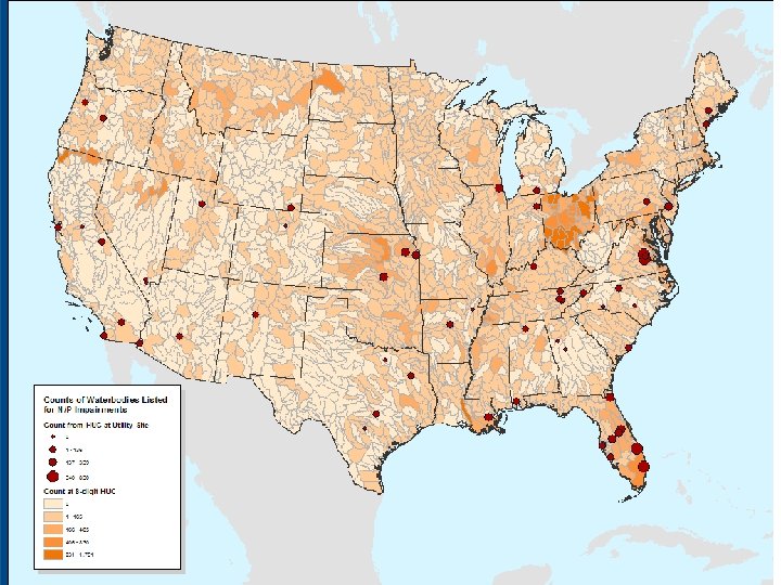
Nutrient pollution is widespread

Water Utilities • 97% of nation’s 160, 000 public water systems serve fewer than 10, 000 persons; 78% of nation’s 15, 000 wastewater treatment plants produce less than one million gallons/day • Face the challenge of providing affordable water services that meet federal and state regulations • Deal with excess nitrogen and phosphate released to the environment by sources such as crop/livestock operations: fertilizers and manure storage • Rural water utilities are smaller, face lower network densities and have a larger number of public firms (sections of the country where private firms do not find it profitable to bring service)

Summary Statistics Spatial Distance Functions Variable Units Mean Std. Dev. Min Max Latitude Decimal (6) 35. 80 6. 20 18. 38 61. 19 Longitude Decimal (6) -93. 14 16. 93 -149. 90 -66. 31 Drinking Water (Y 1) MGD 45. 89 86. 30 1. 35 617 Treated Water (Y 2) MGD 29. 75 42. 04 0. 49 242 Labor (L) Staff 375. 36 748. 97 5 4989 Capital (K) Million $ 463. 17 778. 87 0. 39 4123 Other (O) Million $ 24. 06 44. 23 0. 61 354

Summary Statistics Spatial Distance Functions Exogenous Variable Units Mean Std. Dev. Min Max Size (dummy) >=100000 0. 551 0. 500 0 1 Ground Raw Million 0. 090 0. 661 0 6. 824 ATTAINS 303 D N/P Impair 119 206 0 830 Discharged N Facilities 21 24 0 116 Discharged P Facilities 22 25 0 132 Balanced panel of 59 mostly public firms observed in 2015 and 2016. Data Sources: American Water Works Association, USEPA

Inverse Distance Spatial Weighting Matrix, W Used spectral normalization to generate a 59 X 59 W matrix Each off-diagonal entry [i, j] in the matrix is equal to 1/(distance between point i and point j). Elements of W (Approximate Distances) minimum > 0 0. 00043 2304. 67 miles mean 0. 0078 128. 77 miles max 0. 69 1. 44 miles

Model We use input and output functions and follow Glass, et al. (2017) in that we use cross sectional means to approximate the unobserved common factors as proposed by Wooldridge (2013) This model is then transformed into a spatial autoregressive (SAR) specification [Lee and Yu (2010 a)]: is an n x 1 vector of spatially lagged errors is i. i. d. across i and t with variance is random effects with mean 0 and variance Is the spatial dependence parameter

lndoi LL Coef. z 0. 10 lndoo LL lny 1 -0. 65 -10. 75 lny 1 y 2 lny 2 -0. 16 -2. 39 y 1 y 2 bar lnlo 0. 14 5. 21 lobar 15688 lnko Coef. z -12. 11 0. 57 7. 45 -8. 61 e-06 -1. 79 lnl --0. 13 -4. 44 2. 94 lnk -0. 16 -3. 59 0. 20 6. 04 lno -0. 52 -8. 88 kobar -0. 004 -1. 58 y 2016 0. 15 4. 49 y 2016 -0. 18 -5. 19 9. 38 6. 54 -13. 09 -33. 59 -1. 42 e-06 -3. 41 1. 76 e-06 5. 34 attains_30 -0. 75 -0. 86 attains_30 -1. 33 -2. 10 size -0. 90 -1. 50 size 0. 79 1. 59 lndoo -0. 34 -2. 20 lndoi 0. 0014 0. 10 e. lndoo 0. 73 4. 48 0. 57 2. 21 0. 50 AIC=52. 23 (14) 0. 36 AIC=27. 80 (14) 0. 10 BIC=91. 02 (14) 0. 11 BIC=66. 59 (14) chi 2(5) = 30. 63 Pr > ch 2 = 0. 000 chi 2(4) = 24. 19 Pr > ch 2 = 0. 000 pg e. lndoi W Test Sp pg W Test Sp

lndoi Coef. LL 1. 25 lny 1 -0. 68 z lndoo LL -10. 53 lny 1 y 2 Coef. z -12. 22 0. 60 7. 51 -7. 11 e-06 -1. 58 lny 2 -0. 15 -2. 17 y 1 y 2 bar lnlo 0. 14 5. 09 lnl --0. 14 -4. 78 lobar 16071 3. 08 lnk -0. 18 -4. 07 lnko 0. 19 5. 43 lno -0. 54 -9. 91 kobar -0. 004 -1. 62 y 2016 0. 16 4. 71 y 2016 -0. 18 -5. 02 10. 09 8. 05 -12. 88 -32. 96 -1. 57 e-06 -3. 90 1. 64 e-06 4. 86 n_dmr -0. 12 -0. 74 n_dmr 0. 36 2. 61 p_dmr 0. 12 0. 74 p_dmr -0. 35 -2. 62 size -1. 18 -2. 08 size 0. 38 0. 96 lndoo -0. 30 -1. 71 lndoi 0. 038 1. 36 e. lndoo 0. 72 4. 27 e. lndoi 0. 56 2. 10 0. 48 AIC=54. 45 (df=15) 0. 34 AIC=27. 50 (df=15) 0. 10 BIC=96. 00 (df=15) chi 2(6) = 30. 50 Pr > ch 2 = 0. 0000 pg 0. 11 W Test Sp chi 2(6) = 31. 78 pg BIC=69. 06 (df=15) Pr > ch 2 = 0. 000 W Test Sp

Predicted Efficiencies Calculations predict beta_lndoi (input-oriented inefficiency) beta_doi = exp( beta_lndoi)*o beta_doi 2 = beta_doi/min_ beta_doi efficiency input-oriented = 1/ beta_doi 2 predict beta_lndoo (output-oriented inefficiency) beta_doo = exp( beta_lndoo)*y 2 beta_doo 2 = beta_doo/max_ beta_doo efficiency input-oriented = beta_doo 2

Predicted Efficiency Results Difference in Means (Tests Two-sample t test with unequal variances) Number of Observations in Parentheses Model 1 Model 2 Model 3 Model 4 Mean 0. 40 0. 26 0. 52 0. 26 Std. Dev. 0. 16 0. 13 0. 19 0. 14 Min 0. 13 0. 04 0. 16 0. 05 Max 1 1 Attains_30 d 0. 43(90) 0. 32(28) 0. 55 (90) 0. 42 (28) Metro 0. 13 (8) 0. 26 (110) Size 0. 20 (53) 0. 30 (65) 0. 55 (53) 0. 49 (65) 0. 21 (53) 0. 31 (65) 0. 29 (52) 0. 23 (66) 0. 60 (52) 0. 45 (66) 0. 30 (52) 0. 24 (66) Ratio 0. 48(52) 0. 34(66) Significance: 1% 0. 15 (8) 0. 27 (110) 5% 10%

Ray Scale Economies Calculations Definition for input-oriented distance function. Definition for output-oriented distance function.

Scale Economies Results Ray Input Model 1 1. 23 Model 2 Model 3 Model 4 Ray Output 1. 23 1. 20 1. 17

Average Marginal Effects (z in parentheses) Model 1 Model 2 Model 3 Model 4 Attains_30 -0. 61 (-2. 10) -0. 28 (-0. 89) Size 0. 36 (1. 58) -0. 33 (-1. 58) 0. 18 (0. 94) -0. 45 (-2. 47) PG 8. 06 e-07 (5. 16) -5. 27 e-07 (-3. 31) 7. 71 e-07 (4. 20) -5. 97 e-07 (-2. 62) -0. 18 (-5. 18) 0. 13 (4. 32) -0. 18 (-4. 99) 0. 14 (4. 59) Has_n_dmr 0. 17 (2. 54) -0. 05 (-0. 75) Has_p_dmr -0. 16 (-2. 56) -0. 05 (-0. 75) Y 2016 Significance: 1% 5%

Impact Calculations Total Impact in a vector framework, Y, X, S and W Direct Impact , Indirect Impact

Average Impacts (order: direct, indirect, total) Attains_30 PG Y 2016 Model 1 Model 2 Model 3 Model 4 -0. 00 -0. 61 -0. 01 -0. 29 -0. 28 1. 51 e-10 8. 06 e-07 2. 68 e-08 -5. 54 e-07 -5. 27 e-07 3. 76 e-09 7. 67 e-07 7. 71 e-07 2. 58 e-08 -6. 23 e 07 -5. 97 e-07 -0. 18 -0. 00. -0. 18 0. 15 -0. 02 0. 13 -0. 18 0. 00 -0. 18 0. 16 -0. 02 0. 14 0. 00 -0. 16 10% 0. 02 -0. 47 -0. 45 Has_p_dmr Significance: 1% 5%

Summary of Results • Estimated four distance functions that met the basic theoretical properties. Two input-oriented and two output-oriented. Derived predicted environmental efficiency from these estimations. • Environmental factors such as water bodies impaired by N and P were highly significant in explaining environmental performance. • Scale economies are increasing for the sector. • Location matters also from the standpoint that water utilities located in non-metro areas are less efficient.

Questions? Suggestions? THANK YOU!!!