Spatial Econometric Analysis Using GAUSS 8 KuanPin Lin

Spatial Econometric Analysis Using GAUSS 8 Kuan-Pin Lin Portland State University

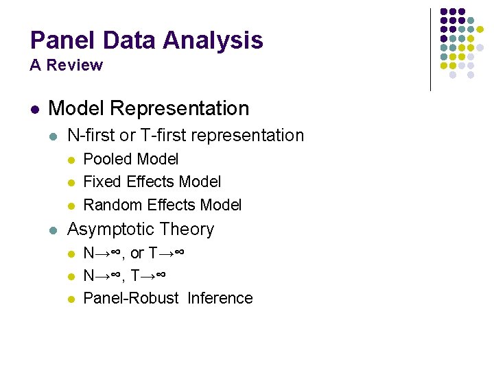
Panel Data Analysis A Review l Model Representation l N-first or T-first representation l l Pooled Model Fixed Effects Model Random Effects Model Asymptotic Theory l l l N→∞, or T→∞ N→∞, T→∞ Panel-Robust Inference

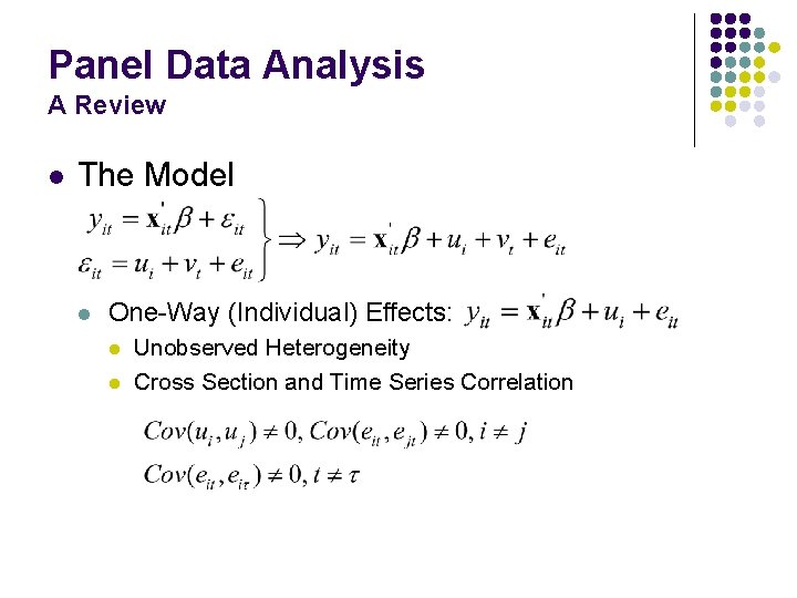
Panel Data Analysis A Review l The Model l One-Way (Individual) Effects: l l Unobserved Heterogeneity Cross Section and Time Series Correlation

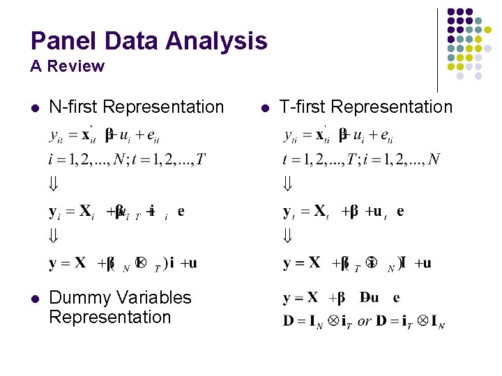
Panel Data Analysis A Review l N-first Representation l Dummy Variables Representation l T-first Representation

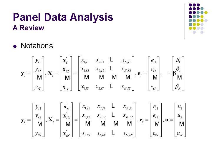
Panel Data Analysis A Review l Notations

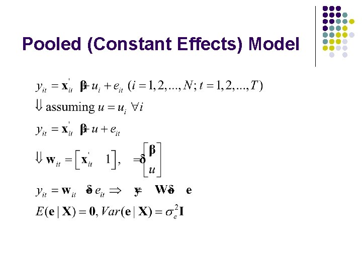
Pooled (Constant Effects) Model

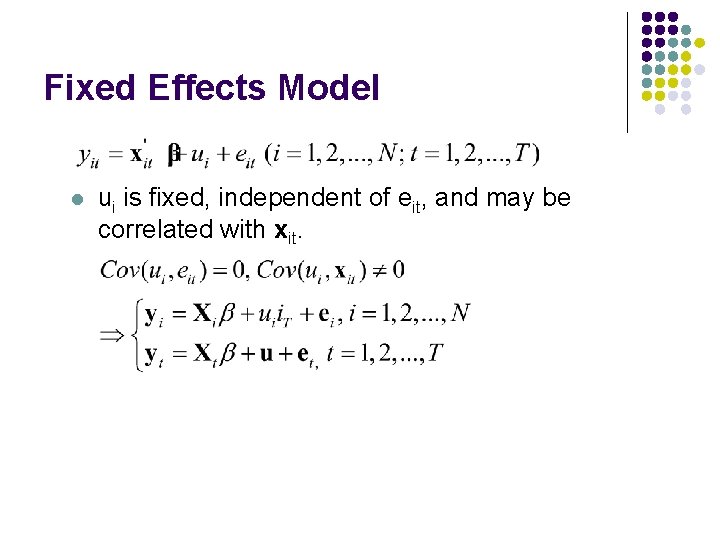
Fixed Effects Model l ui is fixed, independent of eit, and may be correlated with xit.

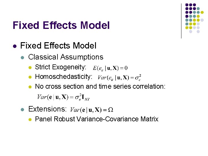
Fixed Effects Model l Classical Assumptions l l Strict Exogeneity: Homoschedasticity: No cross section and time series correlation: Extensions: l Panel Robust Variance-Covariance Matrix

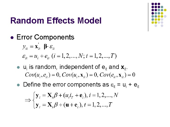
Random Effects Model l Error Components l ui is random, independent of eit and xit. l Define the error components as eit = ui + eit

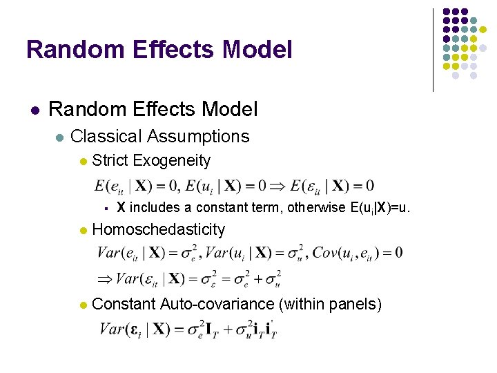
Random Effects Model l Classical Assumptions l Strict Exogeneity § X includes a constant term, otherwise E(ui|X)=u. l Homoschedasticity l Constant Auto-covariance (within panels)

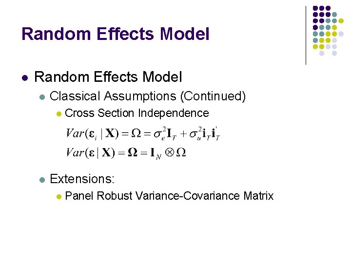
Random Effects Model l Classical Assumptions (Continued) l l Cross Section Independence Extensions: l Panel Robust Variance-Covariance Matrix

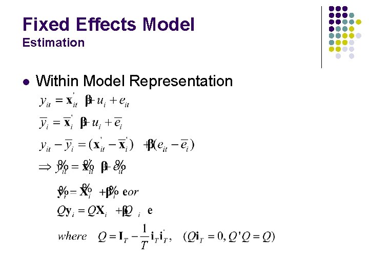
Fixed Effects Model Estimation l Within Model Representation

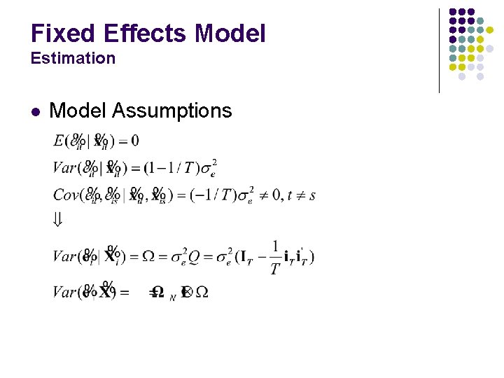
Fixed Effects Model Estimation l Model Assumptions

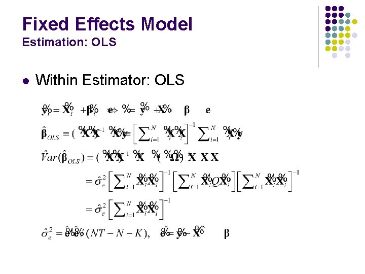
Fixed Effects Model Estimation: OLS l Within Estimator: OLS

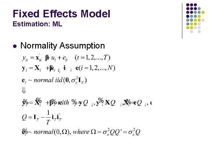
Fixed Effects Model Estimation: ML l Normality Assumption

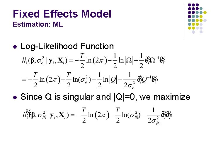
Fixed Effects Model Estimation: ML l Log-Likelihood Function l Since Q is singular and |Q|=0, we maximize

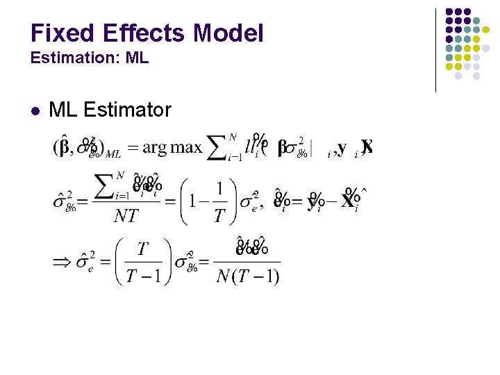
Fixed Effects Model Estimation: ML l ML Estimator

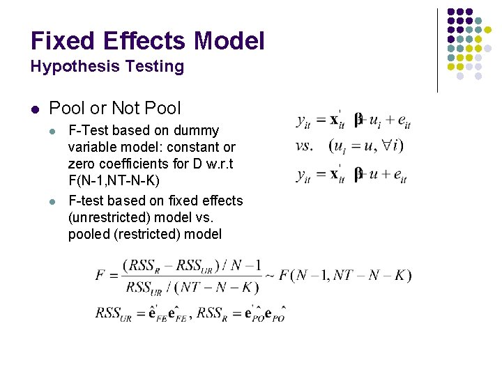
Fixed Effects Model Hypothesis Testing l Pool or Not Pool l l F-Test based on dummy variable model: constant or zero coefficients for D w. r. t F(N-1, NT-N-K) F-test based on fixed effects (unrestricted) model vs. pooled (restricted) model

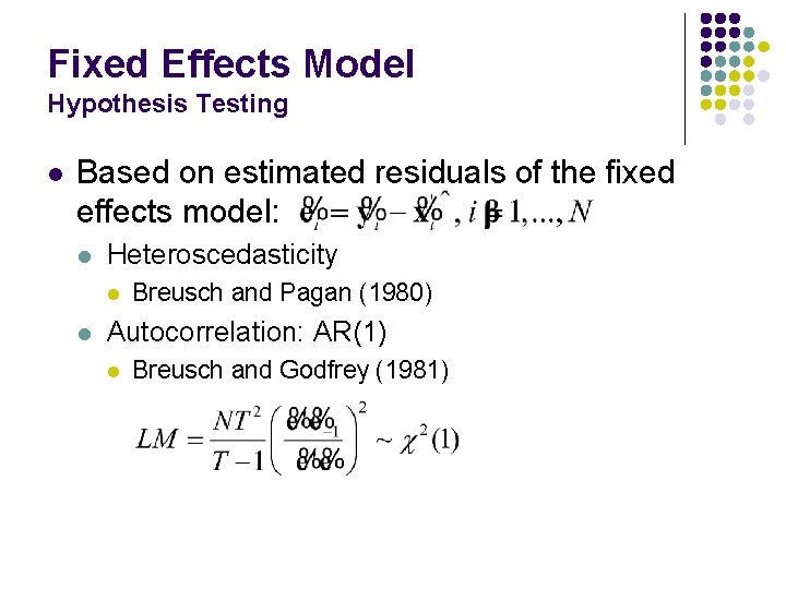
Fixed Effects Model Hypothesis Testing l Based on estimated residuals of the fixed effects model: l Heteroscedasticity l l Breusch and Pagan (1980) Autocorrelation: AR(1) l Breusch and Godfrey (1981)

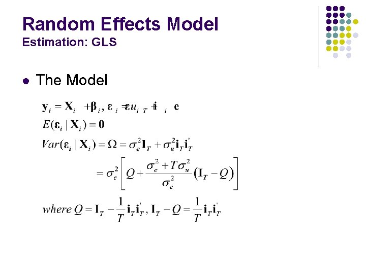
Random Effects Model Estimation: GLS l The Model

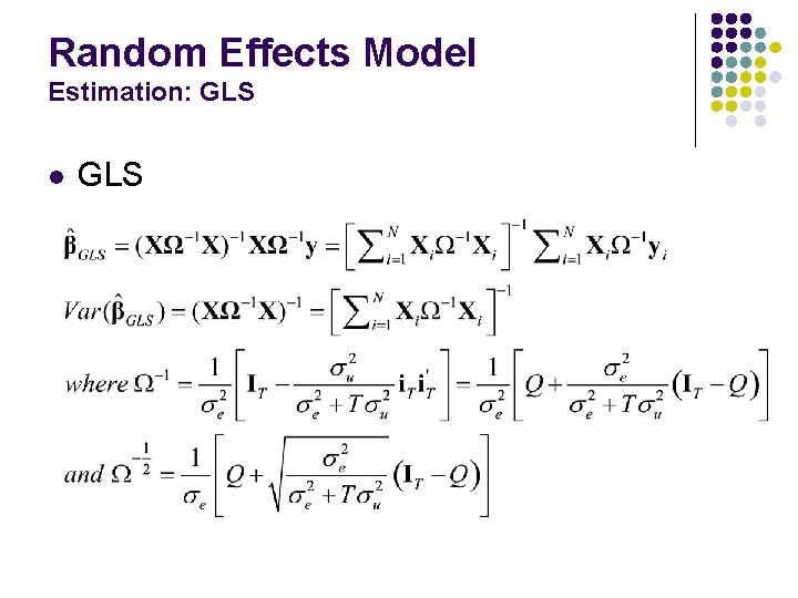
Random Effects Model Estimation: GLS l GLS

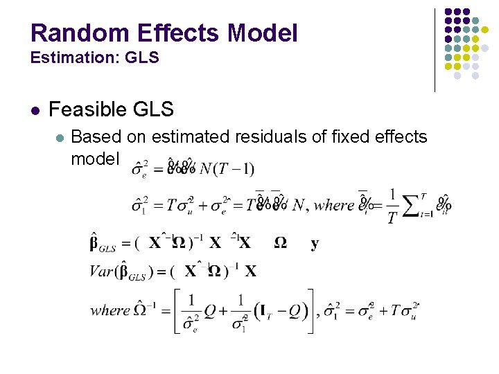
Random Effects Model Estimation: GLS l Feasible GLS l Based on estimated residuals of fixed effects model

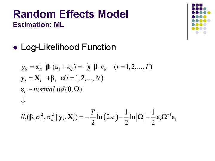
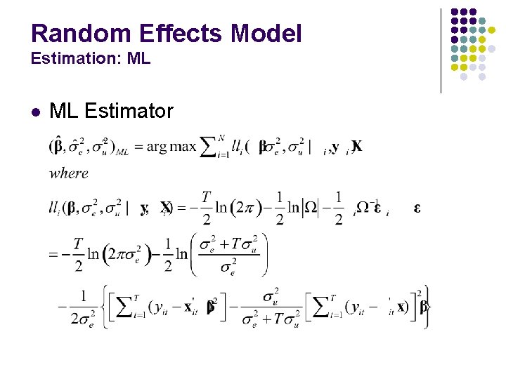
Random Effects Model Estimation: ML l Log-Likelihood Function

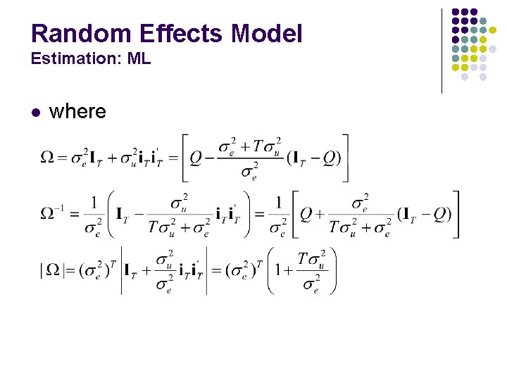
Random Effects Model Estimation: ML l where

Random Effects Model Estimation: ML l ML Estimator

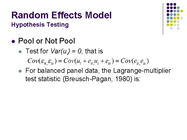
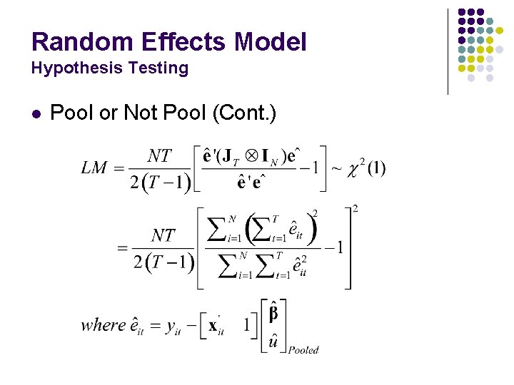
Random Effects Model Hypothesis Testing l Pool or Not Pool l Test for Var(ui) = 0, that is l For balanced panel data, the Lagrange-multiplier test statistic (Breusch-Pagan, 1980) is:

Random Effects Model Hypothesis Testing l Pool or Not Pool (Cont. )

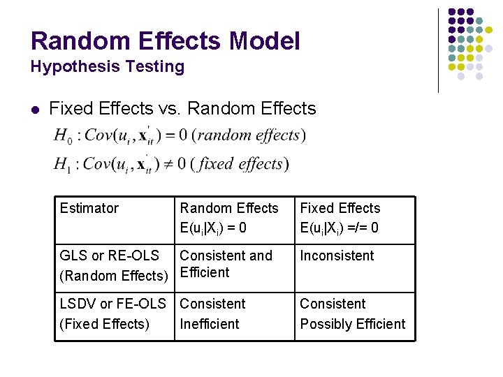
Random Effects Model Hypothesis Testing l Fixed Effects vs. Random Effects Estimator Random Effects E(ui|Xi) = 0 Fixed Effects E(ui|Xi) =/= 0 GLS or RE-OLS Consistent and (Random Effects) Efficient Inconsistent LSDV or FE-OLS Consistent (Fixed Effects) Inefficient Consistent Possibly Efficient

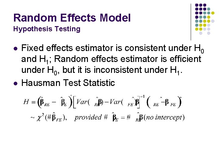
Random Effects Model Hypothesis Testing l l Fixed effects estimator is consistent under H 0 and H 1; Random effects estimator is efficient under H 0, but it is inconsistent under H 1. Hausman Test Statistic

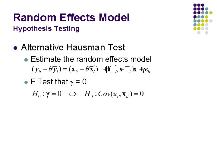
Random Effects Model Hypothesis Testing l Alternative Hausman Test l Estimate the random effects model l F Test that g = 0

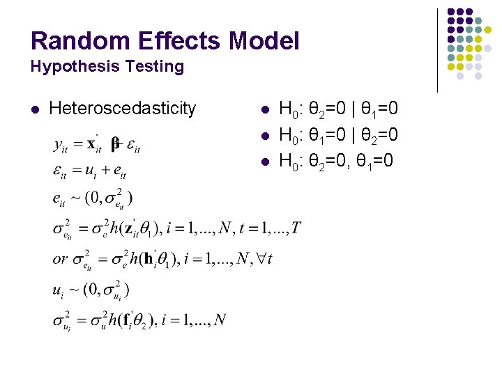
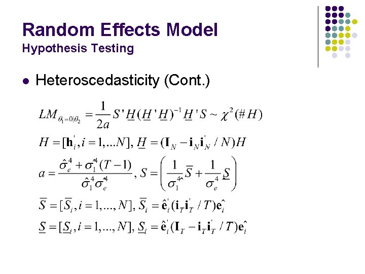
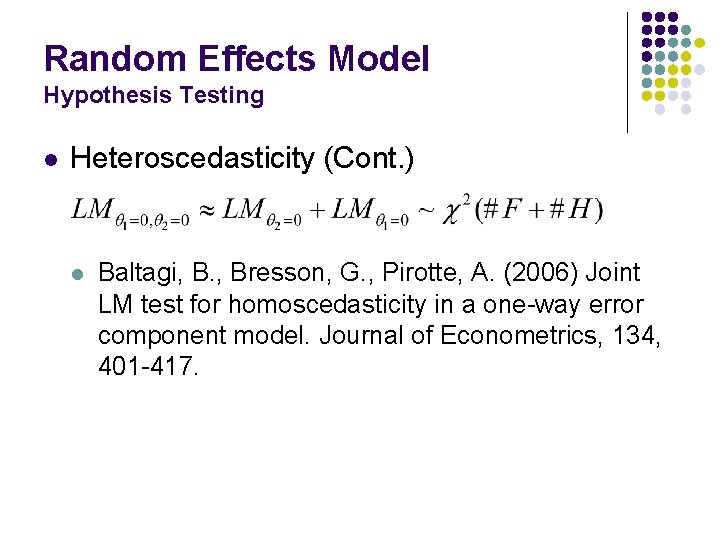
Random Effects Model Hypothesis Testing l Heteroscedasticity l l l H 0: θ 2=0 | θ 1=0 H 0: θ 1=0 | θ 2=0 H 0: θ 2=0, θ 1=0

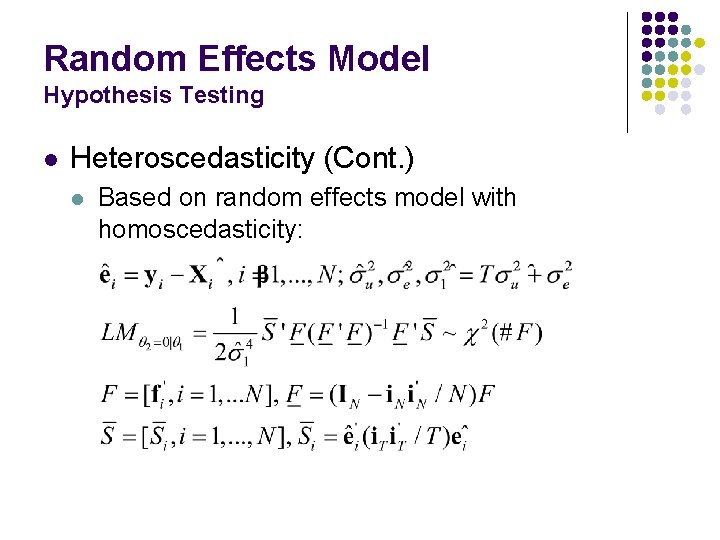
Random Effects Model Hypothesis Testing l Heteroscedasticity (Cont. ) l Based on random effects model with homoscedasticity:

Random Effects Model Hypothesis Testing l Heteroscedasticity (Cont. )

Random Effects Model Hypothesis Testing l Heteroscedasticity (Cont. ) l Baltagi, B. , Bresson, G. , Pirotte, A. (2006) Joint LM test for homoscedasticity in a one-way error component model. Journal of Econometrics, 134, 401 -417.

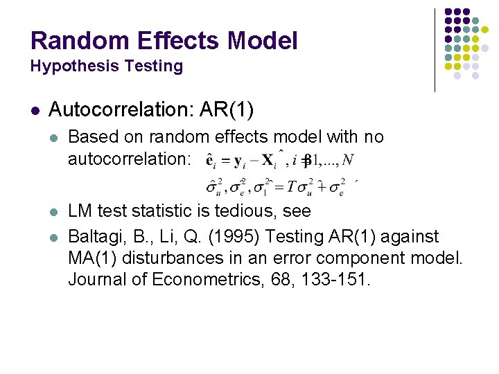
Random Effects Model Hypothesis Testing l Autocorrelation: AR(1) l Based on random effects model with no autocorrelation: l LM test statistic is tedious, see Baltagi, B. , Li, Q. (1995) Testing AR(1) against MA(1) disturbances in an error component model. Journal of Econometrics, 68, 133 -151. l

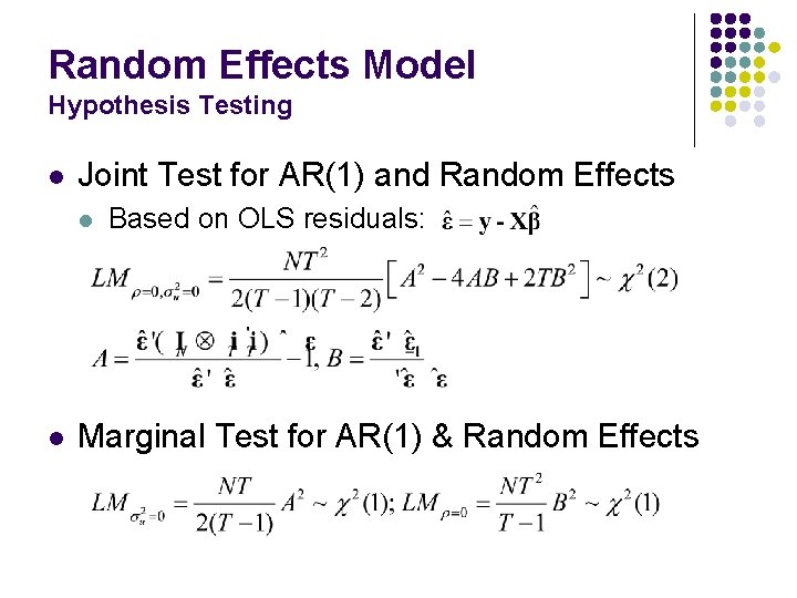
Random Effects Model Hypothesis Testing l Joint Test for AR(1) and Random Effects l l Based on OLS residuals: Marginal Test for AR(1) & Random Effects

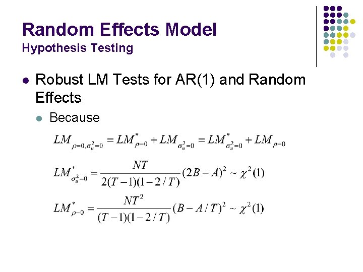
Random Effects Model Hypothesis Testing l Robust LM Tests for AR(1) and Random Effects l Because

Panel Data Analysis An Example: U. S. Productivity l The Model (Munnell [1988]):

Panel Data Analysis An Example: U. S. Productivity l Productivity Data l 48 Continental U. S. States, 17 Years: 1970 -1986 l l l STATE = State name, ST_ABB = State abbreviation, YR = Year, 1970, . . . , 1986, PCAP = Public capital, HWY = Highway capital, WATER = Water utility capital, UTIL = Utility capital, PC = Private capital, GSP = Gross state product, EMP = Employment, UNEMP = Unemployment rate

U. S. Productivity Baltagi (2008) [munnell. 1, munnell. 2] l Panel Data Model ln(GSP) = b 0 + b 1 ln(Public) + b 2 ln(Private) + b 3 ln(Labor) + b 4(Unemp) + e Fixed Effects s. e Random Effects s. e b 1 -0. 026 0. 029 0. 003 0. 024 b 2 0. 292 0. 025 0. 310 0. 020 b 3 0. 768 0. 030 0. 731 0. 026 b 4 -0. 005 0. 001 -0. 006 0. 001 2. 144 0. 137 b 0 F(47, 764) =75. 82 Hausman LM(4) = 905. 1 LM(1) = 4135

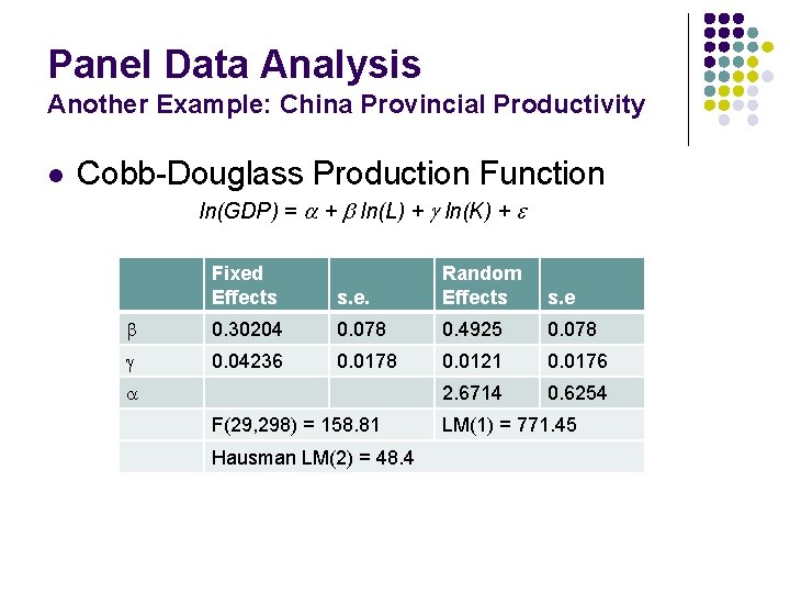
Panel Data Analysis Another Example: China Provincial Productivity l Cobb-Douglass Production Function ln(GDP) = a + b ln(L) + g ln(K) + e Fixed Effects s. e. Random Effects s. e b 0. 30204 0. 078 0. 4925 0. 078 g 0. 04236 0. 0178 0. 0121 0. 0176 2. 6714 0. 6254 a F(29, 298) = 158. 81 Hausman LM(2) = 48. 4 LM(1) = 771. 45

References l l B. H. Baltagi, Econometric Analysis of Panel Data, 4 th ed. , John Wiley, New York, 2008. W. H. Greene, Econometric Analysis, 6 th ed. , Chapter 9: Models for Panel Data, Prentice Hall, 2008. C. Hsiao, Analysis of Panel Data, 2 nd ed. , Cambridge University Press, 2003. J. M. Wooldridge, Econometric Analysis of Cross Section and Panel Data, The MIT Press, 2002.