Spatial Data Mining Outline 1 2 3 4

Spatial Data Mining

Outline 1. 2. 3. 4. 5. Motivation, Spatial Pattern Families Limitations of Traditional Statistics Colocations and Co-occurrences Spatial outliers Summary: What is special about mining spatial data?

Why Data Mining? • Holy Grail - Informed Decision Making • Sensors & Databases increased rate of Data Collection • Transactions, Web logs, GPS-track, Remote sensing, … • Challenges: • Volume (data) >> number of human analysts • Some automation needed • Approaches • Database Querying, e. g. , SQL 3/OGIS • Data Mining for Patterns • …

Data Mining vs. Database Querying • Recall Database Querying (e. g. , SQL 3/OGIS) • Can not answer questions about items not in the database! • Ex. Predict tomorrow’s weather or credit-worthiness of a new customer • Can not efficiently answer complex questions beyond joins • Ex. What are natural groups of customers? • Ex. Which subsets of items are bought together? • Data Mining may help with above questions! • Prediction Models • Clustering, Associations, …

Spatial Data Mining (SDM) • The process of discovering • interesting, useful, non-trivial patterns from large spatial datasets • Spatial pattern families – – – Hotspots, Spatial clusters Spatial outlier, discontinuities Co-locations, co-occurrences Location prediction models …

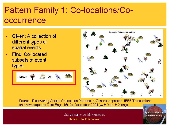
Pattern Family 1: Co-locations/Cooccurrence • Given: A collection of different types of spatial events • Find: Co-located subsets of event types Source: Discovering Spatial Co-location Patterns: A General Approach, IEEE Transactions on Knowledge and Data Eng. , 16(12), December 2004 (w/ H. Yan, H. Xiong).

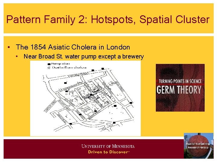
Pattern Family 2: Hotspots, Spatial Cluster • The 1854 Asiatic Cholera in London • Near Broad St. water pump except a brewery

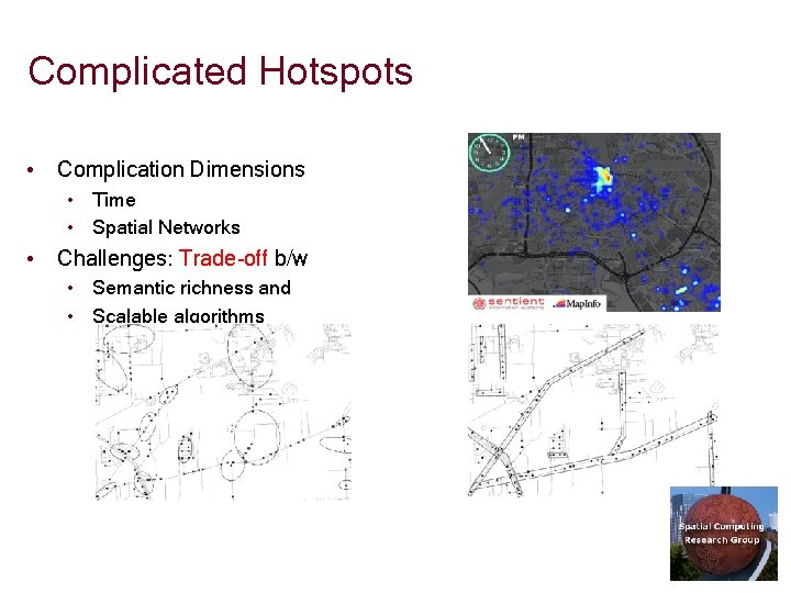
Complicated Hotspots • Complication Dimensions • Time • Spatial Networks • Challenges: Trade-off b/w • Semantic richness and • Scalable algorithms

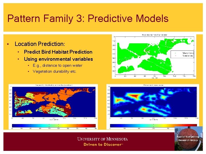
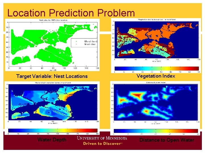
Pattern Family 3: Predictive Models • Location Prediction: • Predict Bird Habitat Prediction • Using environmental variables • E. g. , distance to open water • Vegetation durability etc.

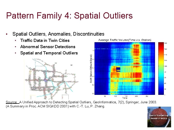
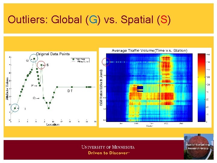
Pattern Family 4: Spatial Outliers • Spatial Outliers, Anomalies, Discontinuities • Traffic Data in Twin Cities • Abnormal Sensor Detections • Spatial and Temporal Outliers Source: A Unified Approach to Detecting Spatial Outliers, Geo. Informatica, 7(2), Springer, June 2003. (A Summary in Proc. ACM SIGKDD 2001) with C. -T. Lu, P. Zhang.

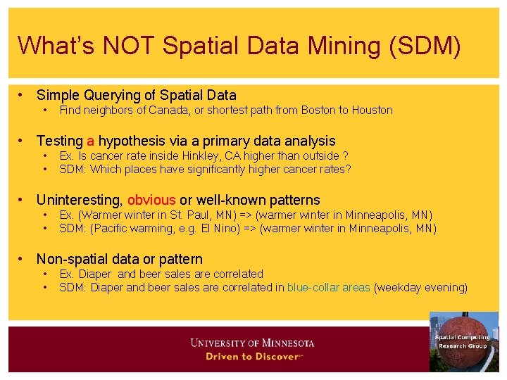
What’s NOT Spatial Data Mining (SDM) • Simple Querying of Spatial Data • Find neighbors of Canada, or shortest path from Boston to Houston • Testing a hypothesis via a primary data analysis • • Ex. Is cancer rate inside Hinkley, CA higher than outside ? SDM: Which places have significantly higher cancer rates? • Uninteresting, obvious or well-known patterns • • Ex. (Warmer winter in St. Paul, MN) => (warmer winter in Minneapolis, MN) SDM: (Pacific warming, e. g. El Nino) => (warmer winter in Minneapolis, MN) • Non-spatial data or pattern • • Ex. Diaper and beer sales are correlated SDM: Diaper and beer sales are correlated in blue-collar areas (weekday evening)

Quiz • Categorize following into queries, hotspots, spatial outlier, colocation, location prediction: (a) Which countries are very different from their neighbors? (b) Which highway-stretches have abnormally high accident rates ? (c) Forecast landfall location for a Hurricane brewing over an ocean? (d) Which retail-store-types often co-locate in shopping malls? (e) What is the distance between Beijing and Chicago?

Limitations of Traditional Statistics • Classical Statistics • Data samples: independent and identically distributed (i. i. d) • Simplifies mathematics underlying statistical methods, e. g. , Linear Regression • Certain amount of “clustering” of spatial events • Spatial data samples are not independent • Spatial Autocorrelation metrics • Global and local Moran’s I • Spatial Heterogeneity • • Spatial data samples may not be identically distributed! No two places on Earth are exactly alike!

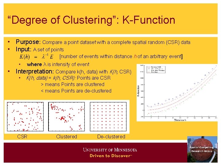
“Degree of Clustering”: K-Function • Purpose: Compare a point dataset with a complete spatial random (CSR) data • Input: A set of points [number of events within distance h of an arbitrary event] • where λ is intensity of event • Interpretation: Compare k(h, data) with K(h, CSR) • K(h, data) = k(h, CSR): Points are CSR > means Points are clustered < means Points are de-clustered CSR Clustered De-clustered

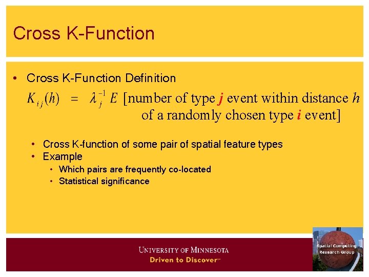
Cross K-Function • Cross K-Function Definition [number of type j event within distance h of a randomly chosen type i event] • Cross K-function of some pair of spatial feature types • Example • Which pairs are frequently co-located • Statistical significance

Estimating K-Function [number of events within distance h of an arbitrary event] [number of type j event within distance h of a randomly chosen type i event]

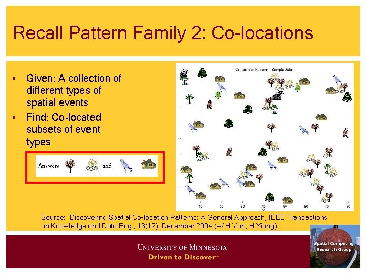
Recall Pattern Family 2: Co-locations • Given: A collection of different types of spatial events • Find: Co-located subsets of event types Source: Discovering Spatial Co-location Patterns: A General Approach, IEEE Transactions on Knowledge and Data Eng. , 16(12), December 2004 (w/ H. Yan, H. Xiong).

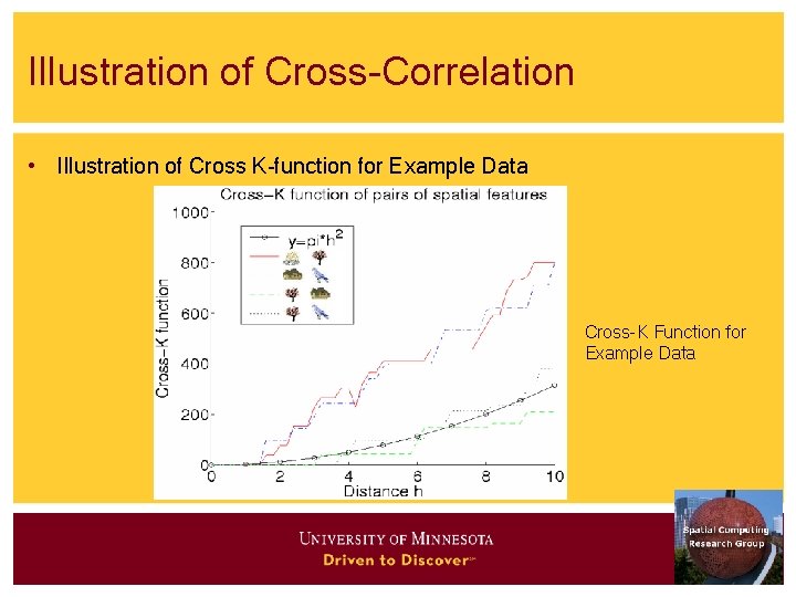
Illustration of Cross-Correlation • Illustration of Cross K-function for Example Data Cross-K Function for Example Data

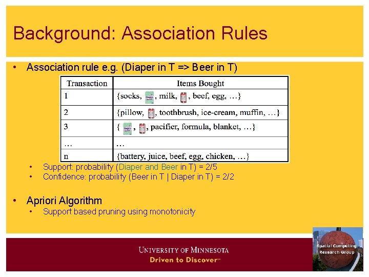
Background: Association Rules • Association rule e. g. (Diaper in T => Beer in T) • • Support: probability (Diaper and Beer in T) = 2/5 Confidence: probability (Beer in T | Diaper in T) = 2/2 • Apriori Algorithm • Support based pruning using monotonicity

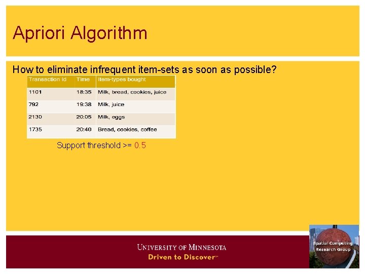
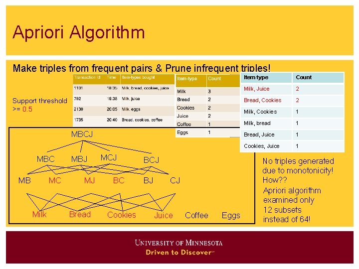
Apriori Algorithm How to eliminate infrequent item-sets as soon as possible? Support threshold >= 0. 5

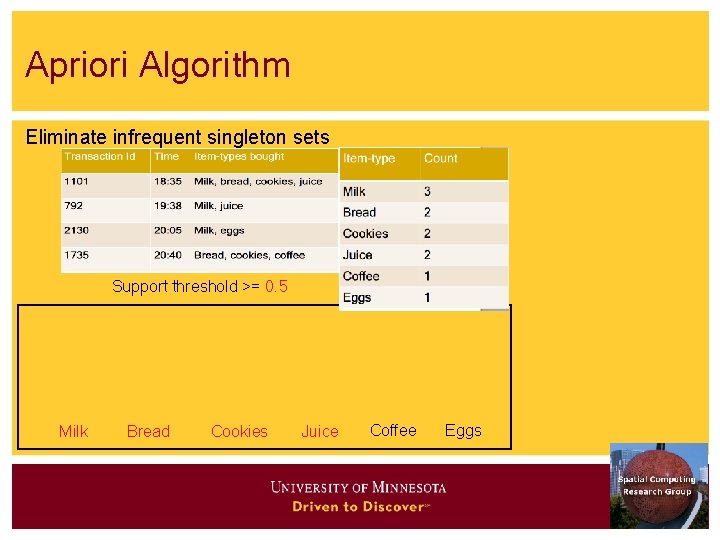
Apriori Algorithm Eliminate infrequent singleton sets Support threshold >= 0. 5 Milk Bread Cookies Juice Coffee Eggs

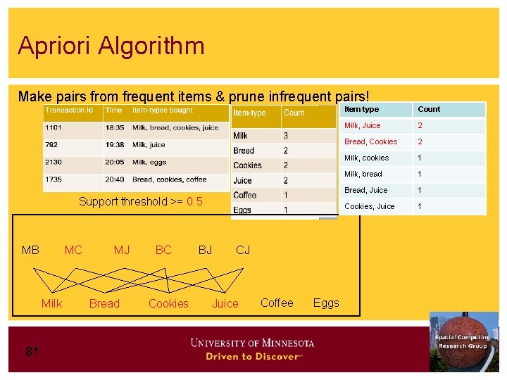
Apriori Algorithm Make pairs from frequent items & prune infrequent pairs! Support threshold >= 0. 5 MB MC Milk 81 MJ Bread BC Cookies BJ CJ Juice Coffee Eggs Item type Count Milk, Juice 2 Bread, Cookies 2 Milk, cookies 1 Milk, bread 1 Bread, Juice 1 Cookies, Juice 1

Apriori Algorithm Make triples from frequent pairs & Prune infrequent triples! Support threshold >= 0. 5 MBCJ MBC MB MC Milk MBJ MJ Bread MCJ BC Cookies BCJ BJ CJ Juice Coffee Eggs Item type Count Milk, Juice 2 Bread, Cookies 2 Milk, Cookies 1 Milk, bread 1 Bread, Juice 1 Cookies, Juice 1 No triples generated due to monotonicity! How? ? Apriori algorithm examined only 12 subsets instead of 64!

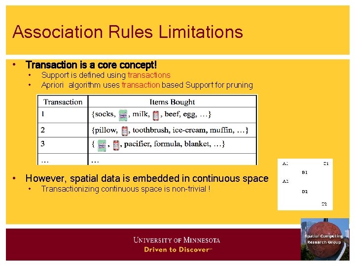
Association Rules Limitations • Transaction is a core concept! • • Support is defined using transactions Apriori algorithm uses transaction based Support for pruning • However, spatial data is embedded in continuous space • Transactionizing continuous space is non-trivial !

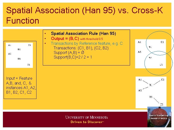
Spatial Association (Han 95) vs. Cross-K Function Input = Feature A, B, and, C, & instances A 1, A 2, B 1, B 2, C 1, C 2 • • Spatial Association Rule (Han 95) Output = (B, C) with threshold 0. 5 • Transactions by Reference feature, e. g. C Transactions: (C 1, B 1), (C 2, B 2) Support (A, B) = Ǿ Support(B, C)=2 / 2 = 1

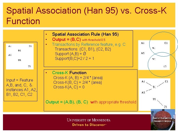
Spatial Association (Han 95) vs. Cross-K Function Input = Feature A, B, and, C, & instances A 1, A 2, B 1, B 2, C 1, C 2 • • Spatial Association Rule (Han 95) Output = (B, C) with threshold 0. 5 • Transactions by Reference feature, e. g. C Transactions: (C 1, B 1), (C 2, B 2) Support (A, B) = Ǿ Support(B, C)=2 / 2 = 1 • Cross-K Function Cross-K (A, B) = 2/4 * (area) Cross-K(B, C) = 2/4 * (area) Cross-K(A, C) = 0 Output = (A, B), (B, C) with appropriate threshold

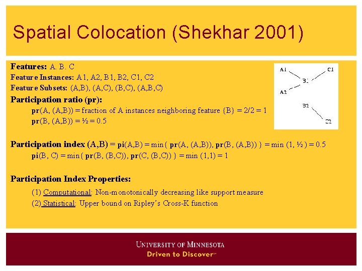
Spatial Colocation (Shekhar 2001) Features: A. B. C Feature Instances: A 1, A 2, B 1, B 2, C 1, C 2 Feature Subsets: (A, B), (A, C), (B, C), (A, B, C) Participation ratio (pr): pr(A, B)) = fraction of A instances neighboring feature {B} = 2/2 = 1 pr(B, (A, B)) = ½ = 0. 5 Participation index (A, B) = pi(A, B) = min{ pr(A, B)), pr(B, (A, B)) } = min (1, ½ ) = 0. 5 pi(B, C) = min{ pr(B, C)), pr(C, (B, C)) } = min (1, 1) = 1 Participation Index Properties: (1) Computational: Non-monotonically decreasing like support measure (2) Statistical: Upper bound on Ripley’s Cross-K function

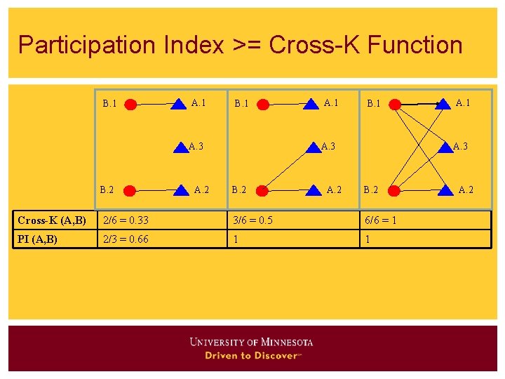
Participation Index >= Cross-K Function B. 1 A. 1 B. 1 A. 3 B. 2 A. 1 A. 3 B. 2 Cross-K (A, B) 2/6 = 0. 33 3/6 = 0. 5 6/6 = 1 PI (A, B) 2/3 = 0. 66 1 1 A. 2

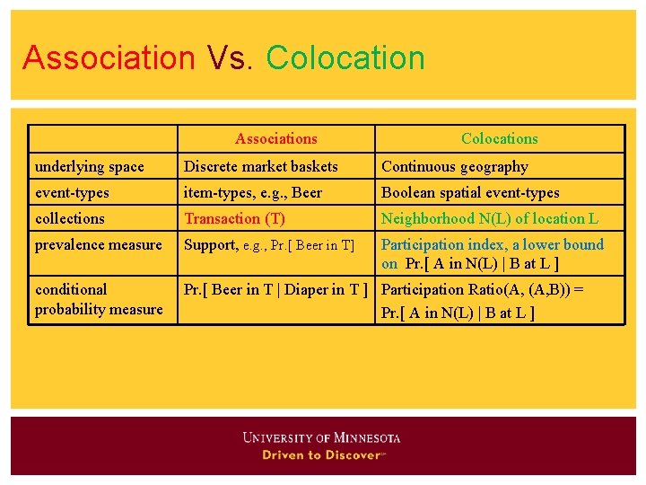
Association Vs. Colocation Associations Colocations underlying space Discrete market baskets Continuous geography event-types item-types, e. g. , Beer Boolean spatial event-types collections Transaction (T) Neighborhood N(L) of location L prevalence measure Support, e. g. , Pr. [ Beer in T] Participation index, a lower bound on Pr. [ A in N(L) | B at L ] conditional probability measure Pr. [ Beer in T | Diaper in T ] Participation Ratio(A, B)) = Pr. [ A in N(L) | B at L ]

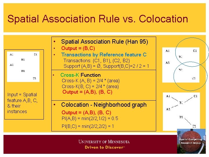
Spatial Association Rule vs. Colocation • Spatial Association Rule (Han 95) • • Output = (B, C) Transactions by Reference feature C Transactions: (C 1, B 1), (C 2, B 2) Support (A, B) = Ǿ, Support(B, C)=2 / 2 = 1 • Cross-K Function Cross-K (A, B) = 2/4 * (area) Cross-K(B, C) = 2/4 * (area) Input = Spatial feature A, B, C, & their instances Output = (A, B), (B, C) • Colocation - Neighborhood graph Output = (A, B), (B, C) PI(A, B) = min(2/2, 1/2) = 0. 5 PI(B, C) = min(2/2, 2/2) = 1

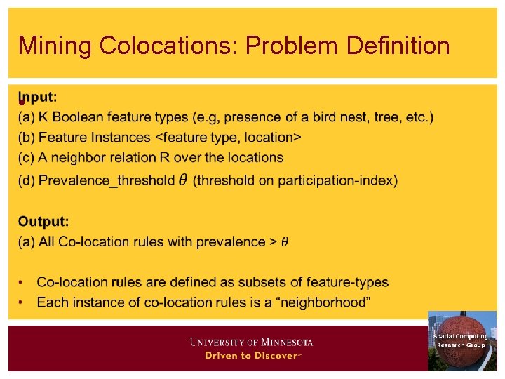
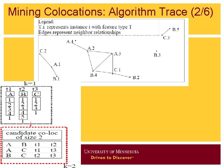
Mining Colocations: Problem Definition •

Key Concepts: Neigborhood

Key Concepts: Co-location rules

Some more Key Concepts

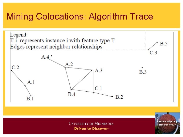
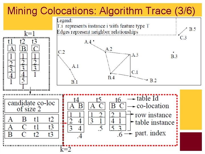
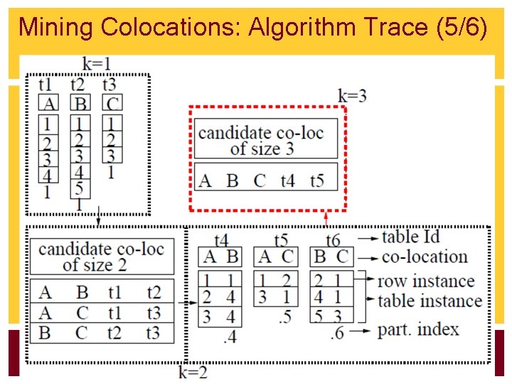
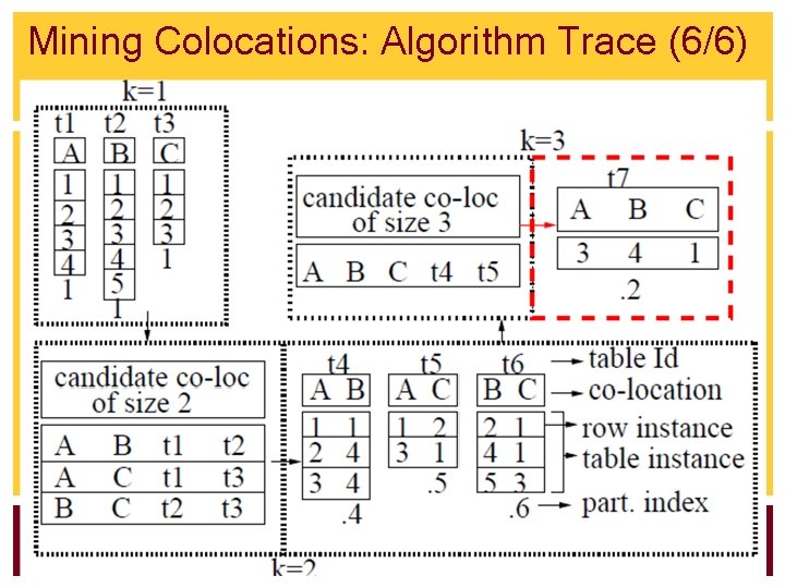
Mining Colocations: Algorithm Trace

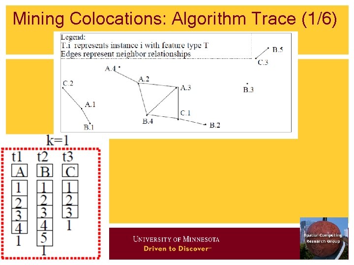
Mining Colocations: Algorithm Trace (1/6)

Mining Colocations: Algorithm Trace (2/6)

Mining Colocations: Algorithm Trace (3/6)

Mining Colocations: Algorithm Trace (5/6)

Mining Colocations: Algorithm Trace (6/6)

Quiz Which is false about concepts underlying association rules? a) Apriori algorithm is used for pruning infrequent item-sets b) Support(diaper, beer) cannot exceed support(diaper) c) Transactions are not natural for spatial data due to continuity of geographic space d) Support(diaper) cannot exceed support(diaper, beer)

Outliers: Global (G) vs. Spatial (S)

Outlier Detection Tests: Variogram Cloud • Graphical Test: Variogram Cloud

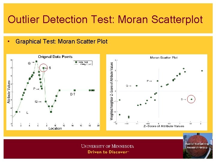
Outlier Detection Test: Moran Scatterplot • Graphical Test: Moran Scatter Plot

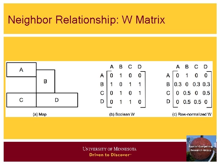
Neighbor Relationship: W Matrix

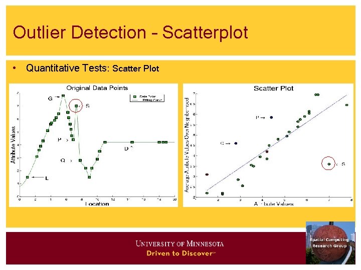
Outlier Detection – Scatterplot • Quantitative Tests: Scatter Plot

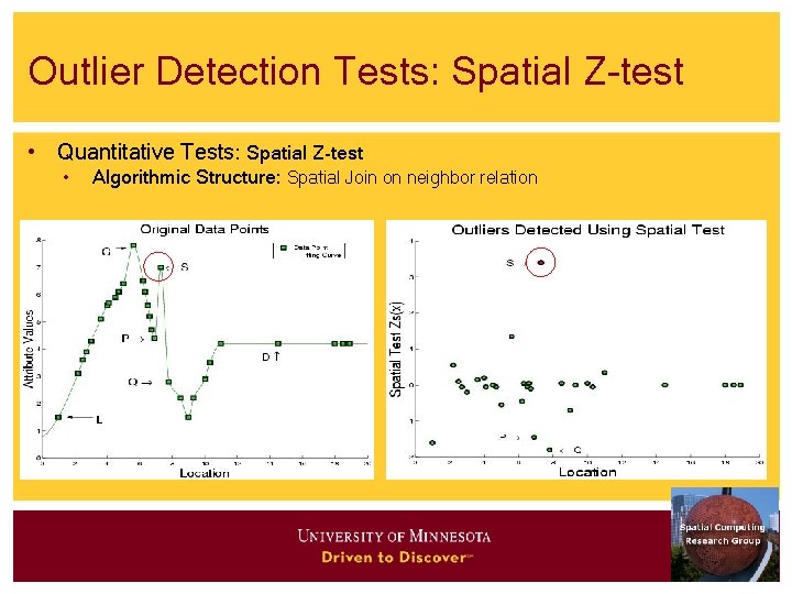
Outlier Detection Tests: Spatial Z-test • Quantitative Tests: Spatial Z-test • Algorithmic Structure: Spatial Join on neighbor relation

Quiz Which of the following is false about spatial outliers? a) Oasis (isolated area of vegetation) is a spatial outlier area in a desert b) They may detect discontinuities and abrupt changes c) They are significantly different from their spatial neighbors d) They are significantly different from entire population

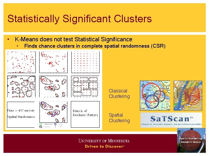
Statistically Significant Clusters • K-Means does not test Statistical Significance • Finds chance clusters in complete spatial randomness (CSR) Classical Clustering Spatial Clustering

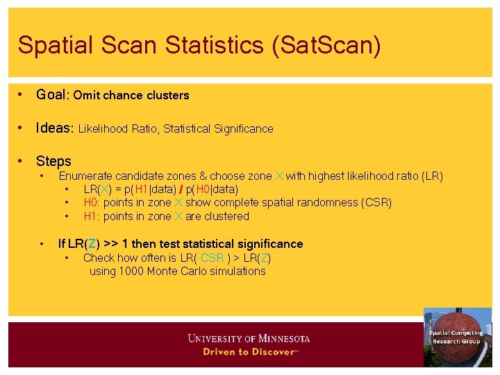
Spatial Scan Statistics (Sat. Scan) • Goal: Omit chance clusters • Ideas: Likelihood Ratio, Statistical Significance • Steps • Enumerate candidate zones & choose zone X with highest likelihood ratio (LR) • LR(X) = p(H 1|data) / p(H 0|data) • H 0: points in zone X show complete spatial randomness (CSR) • H 1: points in zone X are clustered • If LR(Z) >> 1 then test statistical significance • Check how often is LR( CSR ) > LR(Z) using 1000 Monte Carlo simulations

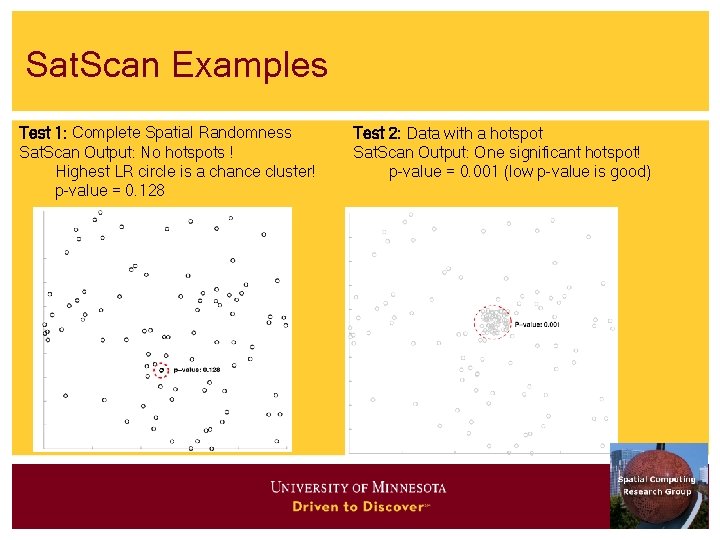
Sat. Scan Examples Test 1: Complete Spatial Randomness Sat. Scan Output: No hotspots ! Highest LR circle is a chance cluster! p-value = 0. 128 Test 2: Data with a hotspot Sat. Scan Output: One significant hotspot! p-value = 0. 001 (low p-value is good)

Location Prediction Problem Target Variable: Nest Locations Water Depth Vegetation Index Distance to Open Water

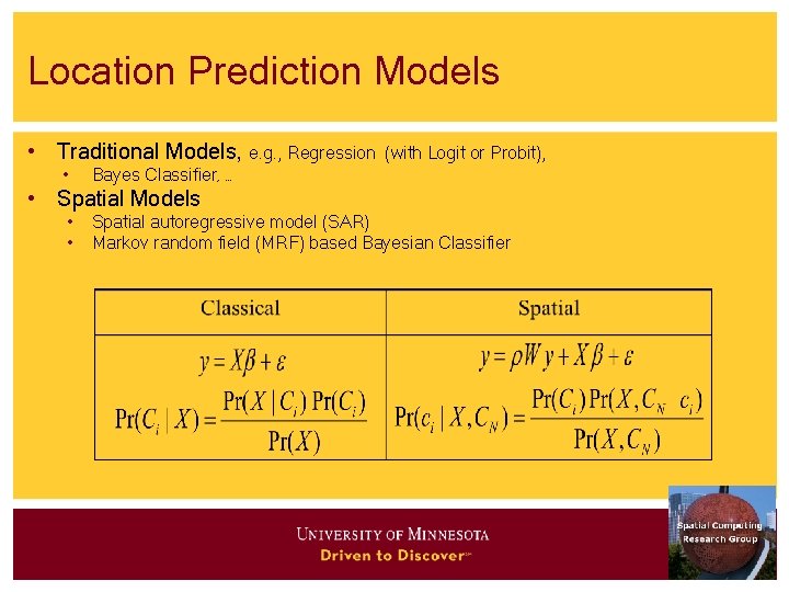
Location Prediction Models • Traditional Models, e. g. , Regression • (with Logit or Probit), Bayes Classifier, … • Spatial Models • • Spatial autoregressive model (SAR) Markov random field (MRF) based Bayesian Classifier