Spatial Data Mining Accomplishments and Research Needs Shashi

Spatial Data Mining: Accomplishments and Research Needs Shashi Shekhar Department of Computer Science and Engineering University of Minnesota

Why Data Mining? n Holy Grail - Informed Decision Making n Lots of Data are Being Collected Business - Transactions, Web logs, GPS-track, … Science - Remote sensing, Micro-array gene expression data, … n Challenges: Volume (data) >> number of human analysts Some automation needed n Data Mining may help! Provide better and customized insights for business Help scientists for hypothesis generation

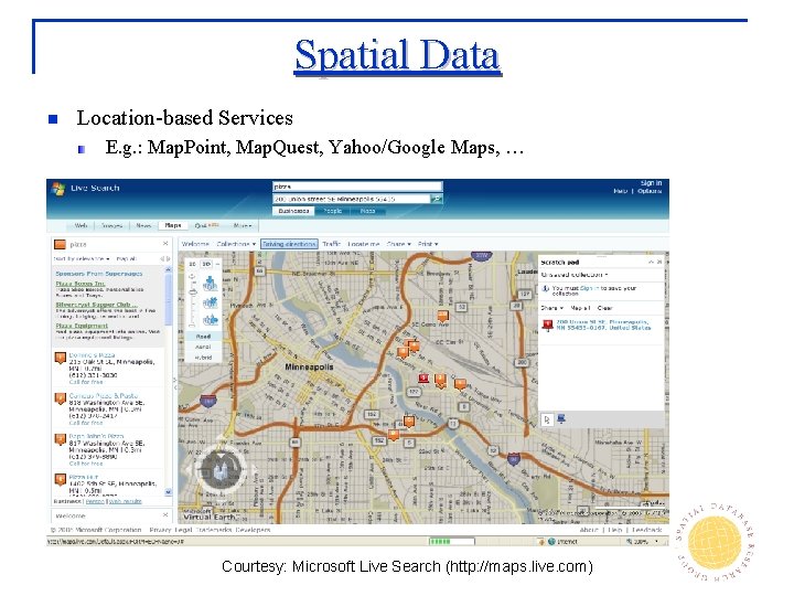
Spatial Data n Location-based Services E. g. : Map. Point, Map. Quest, Yahoo/Google Maps, … Courtesy: Microsoft Live Search (http: //maps. live. com)

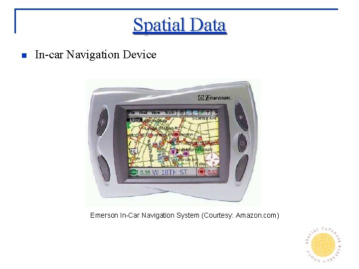
Spatial Data n In-car Navigation Device Emerson In-Car Navigation System (Courtesy: Amazon. com)

Spatial Data Mining (SDM) n The process of discovering interesting, useful, non-trivial patterns Ø Ø patterns: non-specialist exception to patterns: specialist from large spatial datasets n Spatial pattern families Spatial outlier, discontinuities Location prediction models Spatial clusters Co-location patterns …

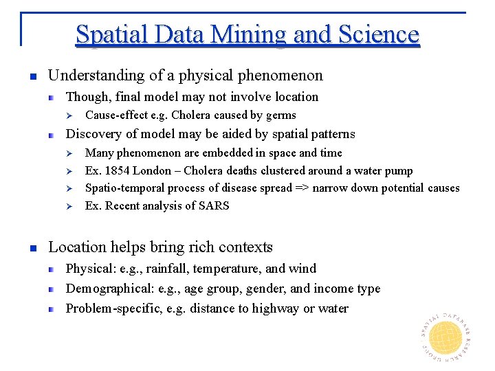
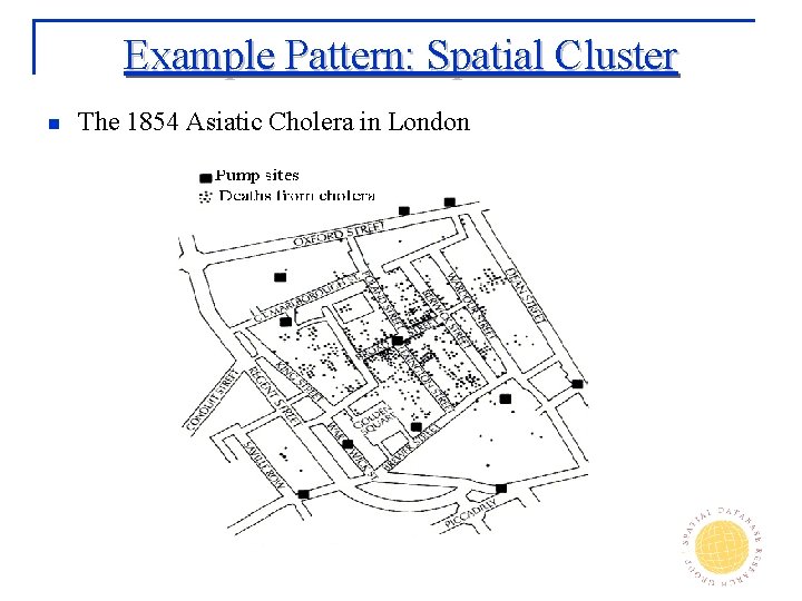
Spatial Data Mining and Science n Understanding of a physical phenomenon Though, final model may not involve location Ø Cause-effect e. g. Cholera caused by germs Discovery of model may be aided by spatial patterns Ø Ø n Many phenomenon are embedded in space and time Ex. 1854 London – Cholera deaths clustered around a water pump Spatio-temporal process of disease spread => narrow down potential causes Ex. Recent analysis of SARS Location helps bring rich contexts Physical: e. g. , rainfall, temperature, and wind Demographical: e. g. , age group, gender, and income type Problem-specific, e. g. distance to highway or water

Example Pattern: Spatial Cluster n The 1854 Asiatic Cholera in London

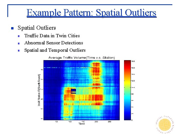
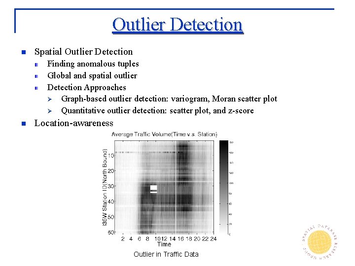
Example Pattern: Spatial Outliers n Spatial Outliers Traffic Data in Twin Cities Abnormal Sensor Detections Spatial and Temporal Outliers

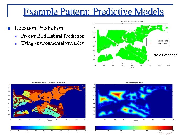
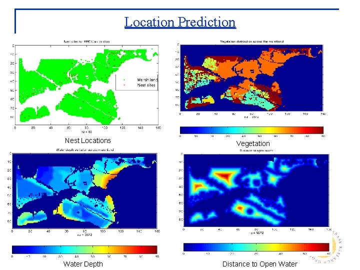
Example Pattern: Predictive Models n Location Prediction: Predict Bird Habitat Prediction Using environmental variables Nest Locations

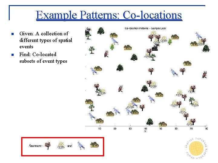
Example Patterns: Co-locations n n Given: A collection of different types of spatial events Find: Co-located subsets of event types

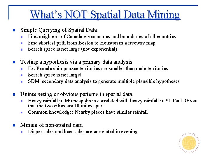
What’s NOT Spatial Data Mining n Simple Querying of Spatial Data Find neighbors of Canada given names and boundaries of all countries Find shortest path from Boston to Houston in a freeway map Search space is not large (not exponential) n Testing a hypothesis via a primary data analysis Ex. Female chimpanzee territories are smaller than male territories Search space is not large! SDM: secondary data analysis to generate multiple plausible hypotheses n Uninteresting or obvious patterns in spatial data Heavy rainfall in Minneapolis is correlated with heavy rainfall in St. Paul, Given that the two cities are 10 miles apart. Common knowledge: Nearby places have similar rainfall n Mining of non-spatial data Diaper sales and beer sales are correlated in evening

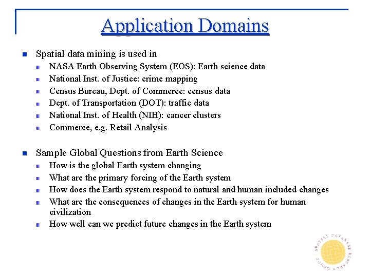
Application Domains n Spatial data mining is used in NASA Earth Observing System (EOS): Earth science data National Inst. of Justice: crime mapping Census Bureau, Dept. of Commerce: census data Dept. of Transportation (DOT): traffic data National Inst. of Health (NIH): cancer clusters Commerce, e. g. Retail Analysis n Sample Global Questions from Earth Science How is the global Earth system changing What are the primary forcing of the Earth system How does the Earth system respond to natural and human included changes What are the consequences of changes in the Earth system for human civilization How well can we predict future changes in the Earth system

Example of Application Domains n Sample Local Questions from Epidemiology [Terra. Seer] What’s overall pattern of colorectal cancer Is there clustering of high colorectal cancer incidence anywhere in the study area Where is colorectal cancer risk significantly elevated Where are zones of rapid change in colorectal cancer incidence Geographic distribution of male colorectal cancer in Long Island, New York (Courtesy: Terra. Seer)

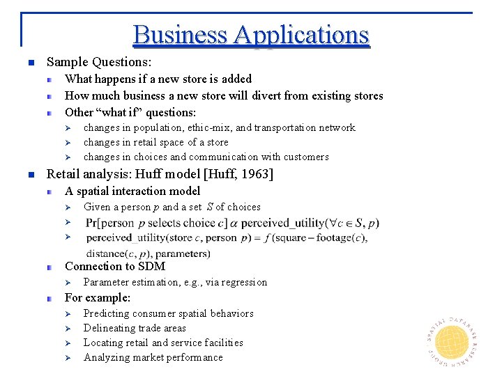
Business Applications n Sample Questions: What happens if a new store is added How much business a new store will divert from existing stores Other “what if” questions: Ø Ø Ø n changes in population, ethic-mix, and transportation network changes in retail space of a store changes in choices and communication with customers Retail analysis: Huff model [Huff, 1963] A spatial interaction model Ø Given a person p and a set S of choices Ø Ø Connection to SDM Ø Parameter estimation, e. g. , via regression For example: Ø Ø Predicting consumer spatial behaviors Delineating trade areas Locating retail and service facilities Analyzing market performance

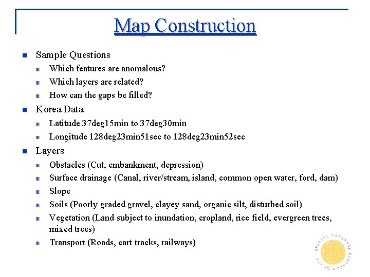
Map Construction n Sample Questions Which features are anomalous? Which layers are related? How can the gaps be filled? n Korea Data Latitude 37 deg 15 min to 37 deg 30 min Longitude 128 deg 23 min 51 sec to 128 deg 23 min 52 sec n Layers Obstacles (Cut, embankment, depression) Surface drainage (Canal, river/stream, island, common open water, ford, dam) Slope Soils (Poorly graded gravel, clayey sand, organic silt, disturbed soil) Vegetation (Land subject to inundation, cropland, rice field, evergreen trees, mixed trees) Transport (Roads, cart tracks, railways)

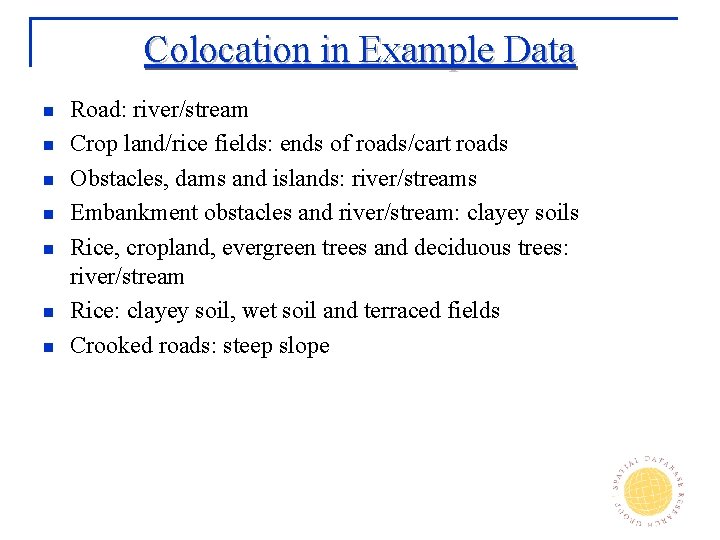
Colocation in Example Data n n n n Road: river/stream Crop land/rice fields: ends of roads/cart roads Obstacles, dams and islands: river/streams Embankment obstacles and river/stream: clayey soils Rice, cropland, evergreen trees and deciduous trees: river/stream Rice: clayey soil, wet soil and terraced fields Crooked roads: steep slope

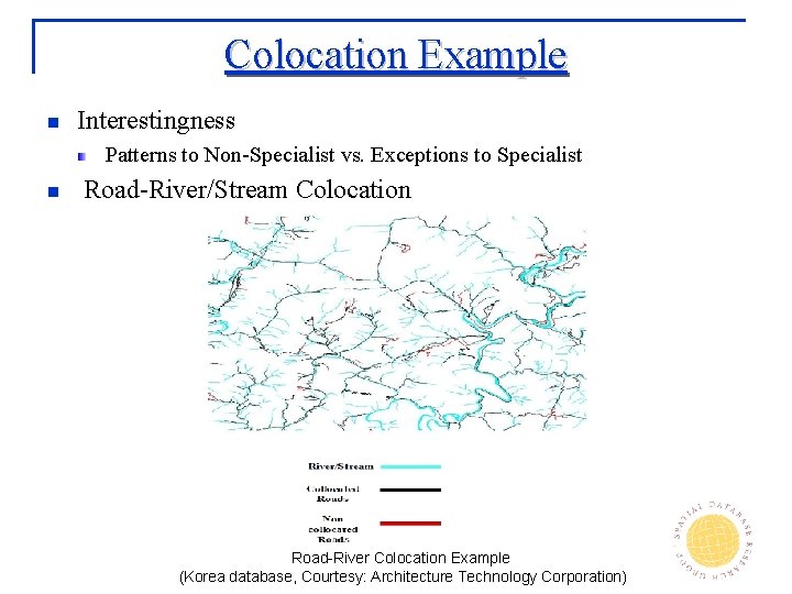
Colocation Example n Interestingness Patterns to Non-Specialist vs. Exceptions to Specialist n Road-River/Stream Colocation Road-River Colocation Example (Korea database, Courtesy: Architecture Technology Corporation)

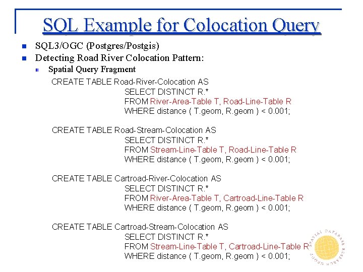
SQL Example for Colocation Query n n SQL 3/OGC (Postgres/Postgis) Detecting Road River Colocation Pattern: Spatial Query Fragment CREATE TABLE Road-River-Colocation AS SELECT DISTINCT R. * FROM River-Area-Table T, Road-Line-Table R WHERE distance ( T. geom, R. geom ) < 0. 001; CREATE TABLE Road-Stream-Colocation AS SELECT DISTINCT R. * FROM Stream-Line-Table T, Road-Line-Table R WHERE distance ( T. geom, R. geom ) < 0. 001; CREATE TABLE Cartroad-River-Colocation AS SELECT DISTINCT R. * FROM River-Area-Table T, Cartroad-Line-Table R WHERE distance ( T. geom, R. geom ) < 0. 001; CREATE TABLE Cartroad-Stream-Colocation AS SELECT DISTINCT R. * FROM Stream-Line-Table T, Cartroad-Line-Table R WHERE distance ( T. geom, R. geom ) < 0. 001;

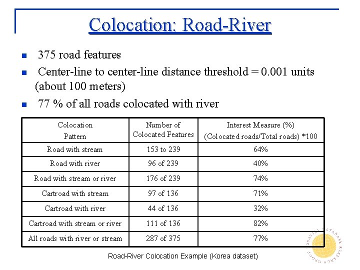
Colocation: Road-River n n n 375 road features Center-line to center-line distance threshold = 0. 001 units (about 100 meters) 77 % of all roads colocated with river Colocation Pattern Number of Colocated Features Interest Measure (%) (Colocated roads/Total roads) *100 Road with stream 153 to 239 64% Road with river 96 of 239 40% Road with stream or river 176 of 239 74% Cartroad with stream 97 of 136 71% Cartroad with river 44 of 136 32% Cartroad with stream or river 111 of 136 82% All roads with river or stream 287 of 375 77% Road-River Colocation Example (Korea dataset)

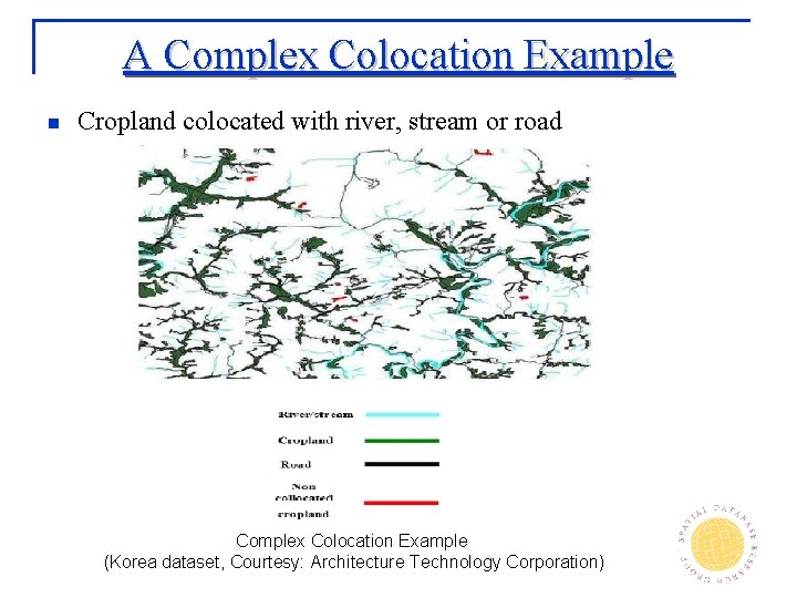
A Complex Colocation Example n Cropland colocated with river, stream or road Complex Colocation Example (Korea dataset, Courtesy: Architecture Technology Corporation)

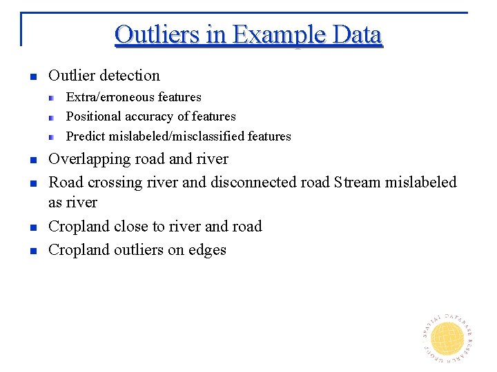
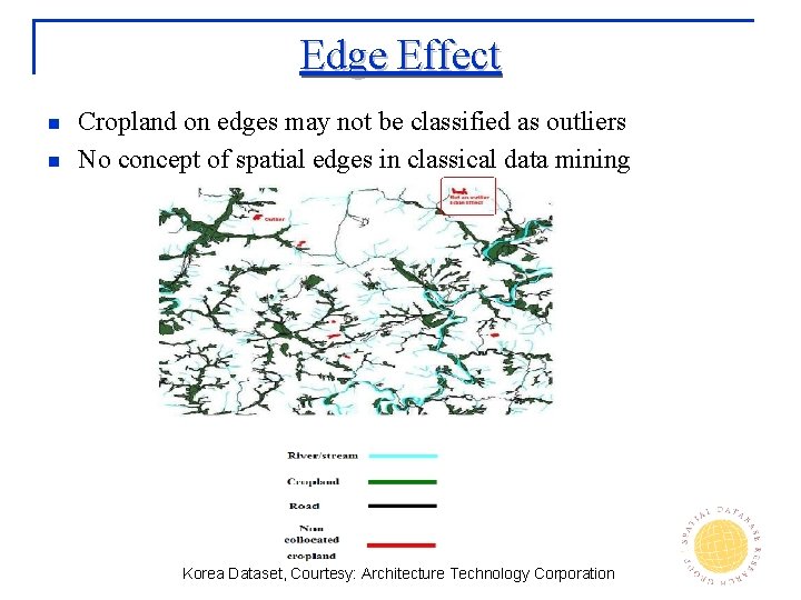
Outliers in Example Data n Outlier detection Extra/erroneous features Positional accuracy of features Predict mislabeled/misclassified features n n Overlapping road and river Road crossing river and disconnected road Stream mislabeled as river Cropland close to river and road Cropland outliers on edges

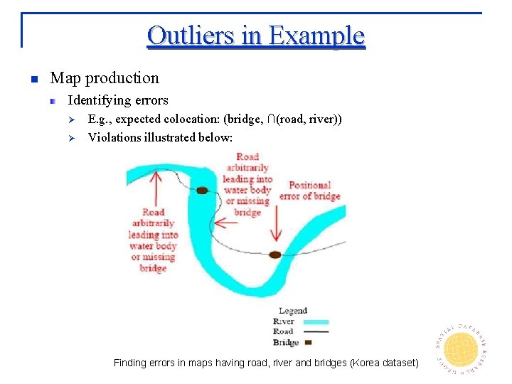
Outliers in Example n Map production Identifying errors Ø Ø E. g. , expected colocation: (bridge, ∩(road, river)) Violations illustrated below: Finding errors in maps having road, river and bridges (Korea dataset)

Overview n Spatial Data Mining Find interesting, potentially useful, non-trivial patterns from spatial data n Components of Data Mining Input: table with many columns, domain (column) Statistical Foundation Output: patterns and interest measures Ø e. g. , predictive models, clusters, outliers, associations Computational process: algorithms

Overview Ø n n Input Statistical Foundation Output Computational Process Trends

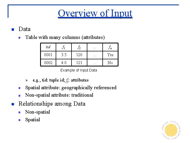
Overview of Input n Data Table with many columns (attributes) tid f 1 f 2 … fn 0001 3. 5 120 … Yes 0002 4. 0 121 … No Example of Input Data Ø e. g. , tid: tuple id; fi: attributes Spatial attribute: geographically referenced Non-spatial attribute: traditional n Relationships among Data Non-spatial Spatial

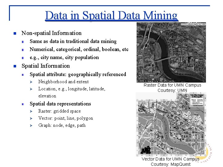
Data in Spatial Data Mining n Non-spatial Information Same as data in traditional data mining Numerical, categorical, ordinal, boolean, etc e. g. , city name, city population n Spatial Information Spatial attribute: geographically referenced Ø Ø Neighborhood and extent Location, e. g. , longitude, latitude, elevation Raster Data for UMN Campus Courtesy: UMN Spatial data representations Ø Ø Ø Raster: gridded space Vector: point, line, polygon Graph: node, edge, path Vector Data for UMN Campus Courtesy: Map. Quest

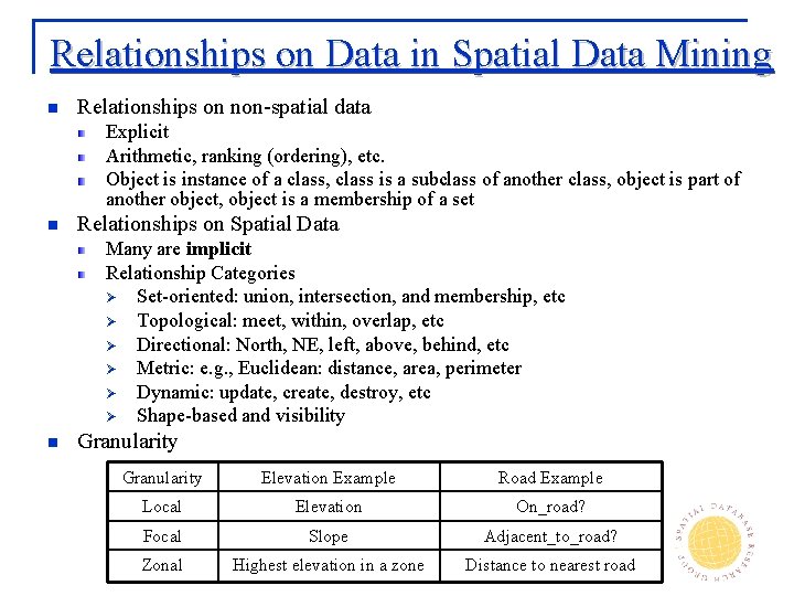
Relationships on Data in Spatial Data Mining n Relationships on non-spatial data Explicit Arithmetic, ranking (ordering), etc. Object is instance of a class, class is a subclass of another class, object is part of another object, object is a membership of a set n Relationships on Spatial Data Many are implicit Relationship Categories Ø Set-oriented: union, intersection, and membership, etc Ø Topological: meet, within, overlap, etc Ø Directional: North, NE, left, above, behind, etc Ø Metric: e. g. , Euclidean: distance, area, perimeter Ø Dynamic: update, create, destroy, etc Ø Shape-based and visibility n Granularity Elevation Example Road Example Local Elevation On_road? Focal Slope Adjacent_to_road? Zonal Highest elevation in a zone Distance to nearest road

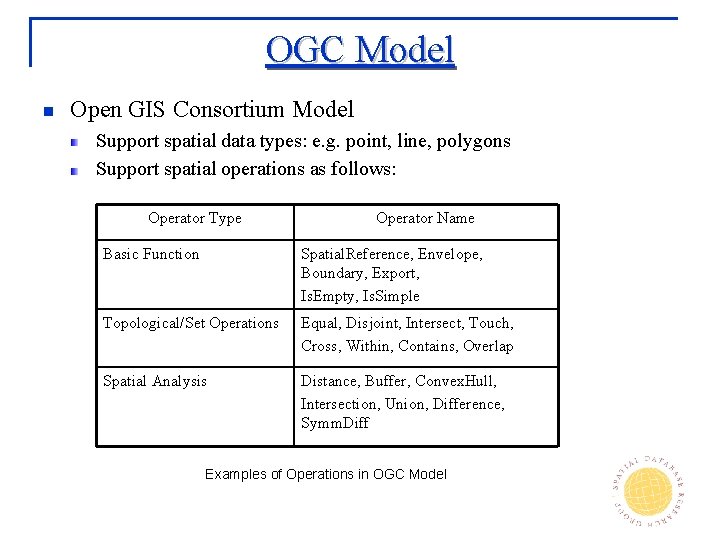
OGC Model n Open GIS Consortium Model Support spatial data types: e. g. point, line, polygons Support spatial operations as follows: Operator Type Operator Name Basic Function Spatial. Reference, Envelope, Boundary, Export, Is. Empty, Is. Simple Topological/Set Operations Equal, Disjoint, Intersect, Touch, Cross, Within, Contains, Overlap Spatial Analysis Distance, Buffer, Convex. Hull, Intersection, Union, Difference, Symm. Diff Examples of Operations in OGC Model

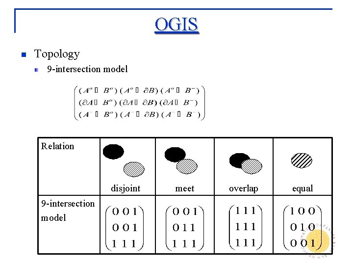
OGIS n Topology 9 -intersection model Relation disjoint 9 -intersection model meet overlap equal

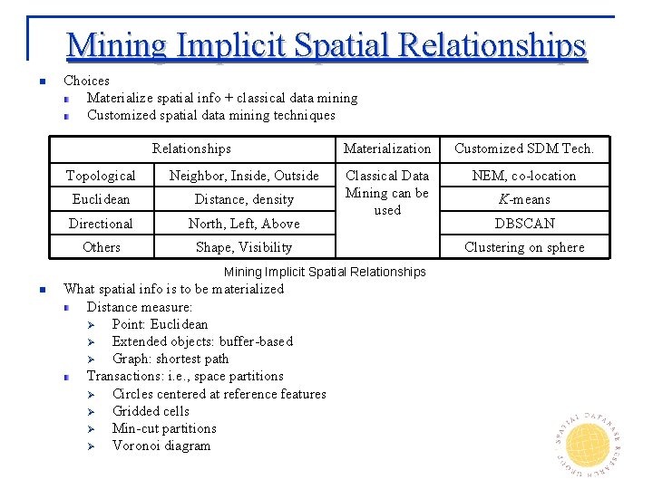
Mining Implicit Spatial Relationships n Choices Materialize spatial info + classical data mining Customized spatial data mining techniques Relationships Topological Neighbor, Inside, Outside Euclidean Distance, density Directional North, Left, Above Others Shape, Visibility Materialization Customized SDM Tech. Classical Data Mining can be used NEM, co-location Mining Implicit Spatial Relationships n What spatial info is to be materialized Distance measure: Ø Point: Euclidean Ø Extended objects: buffer-based Ø Graph: shortest path Transactions: i. e. , space partitions Ø Circles centered at reference features Ø Gridded cells Ø Min-cut partitions Ø Voronoi diagram K-means DBSCAN Clustering on sphere

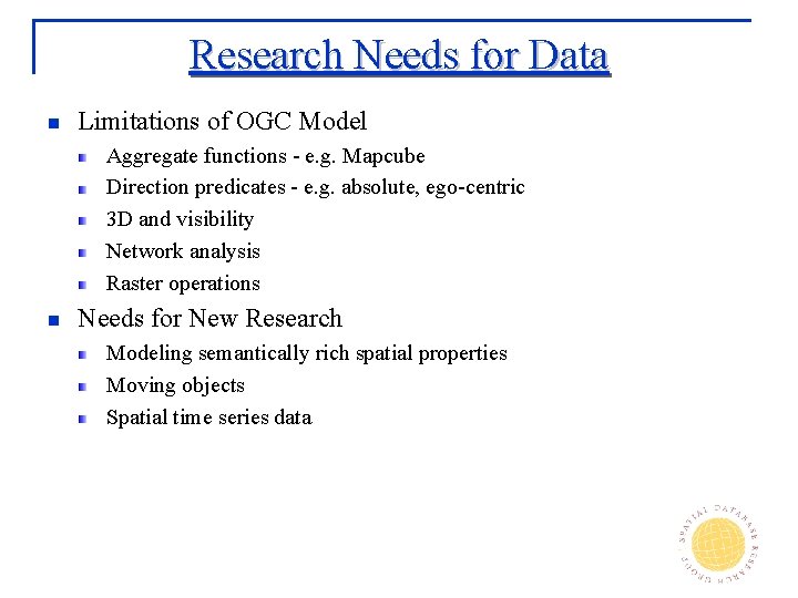
Research Needs for Data n Limitations of OGC Model Aggregate functions - e. g. Mapcube Direction predicates - e. g. absolute, ego-centric 3 D and visibility Network analysis Raster operations n Needs for New Research Modeling semantically rich spatial properties Moving objects Spatial time series data

Overview ü Ø n n n Input Statistical Foundation Output Computational Process Trends

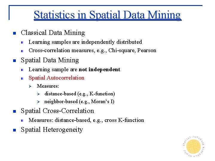
Statistics in Spatial Data Mining n Classical Data Mining Learning samples are independently distributed Cross-correlation measures, e. g. , Chi-square, Pearson n Spatial Data Mining Learning sample are not independent Spatial Autocorrelation Ø n Measures: Ø distance-based (e. g. , K-function) Ø neighbor-based (e. g. , Moran’s I) Spatial Cross-Correlation Measures: distance-based, e. g. , cross K-function n Spatial Heterogeneity

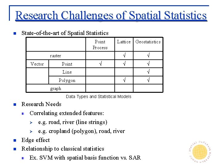
Overview of Statistical Foundation n Spatial Statistics [Cressie, 1991][Hanning, 2003] Geostatistics Ø Continuous Ø Variogram: measure how similarity decreases with distance Ø Spatial interpolation Lattice-based statistics Ø Ø Ø Discrete location, neighbor relationship graph Spatial Gaussian models Ø Conditionally specified, Simultaneously specified spatial Gaussian model Markov Random Fields, Spatial Autoregressive Model Point process Ø Ø Ø Discrete Complete spatial randomness (CSR): Poisson process in space K-function: test of CSR Point Process Lattice Raster Vector Point √ √ √ Line Polygon Graph Geostatistics √ √ √

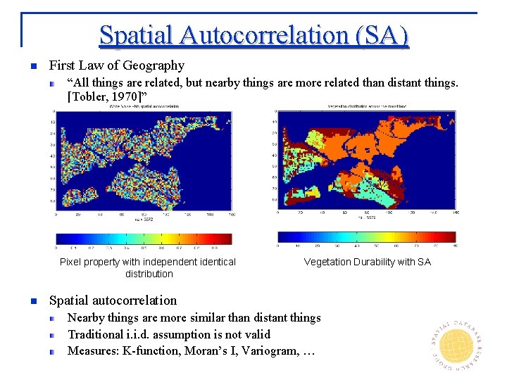
Spatial Autocorrelation (SA) n First Law of Geography “All things are related, but nearby things are more related than distant things. [Tobler, 1970]” Pixel property with independent identical distribution n Vegetation Durability with SA Spatial autocorrelation Nearby things are more similar than distant things Traditional i. i. d. assumption is not valid Measures: K-function, Moran’s I, Variogram, …

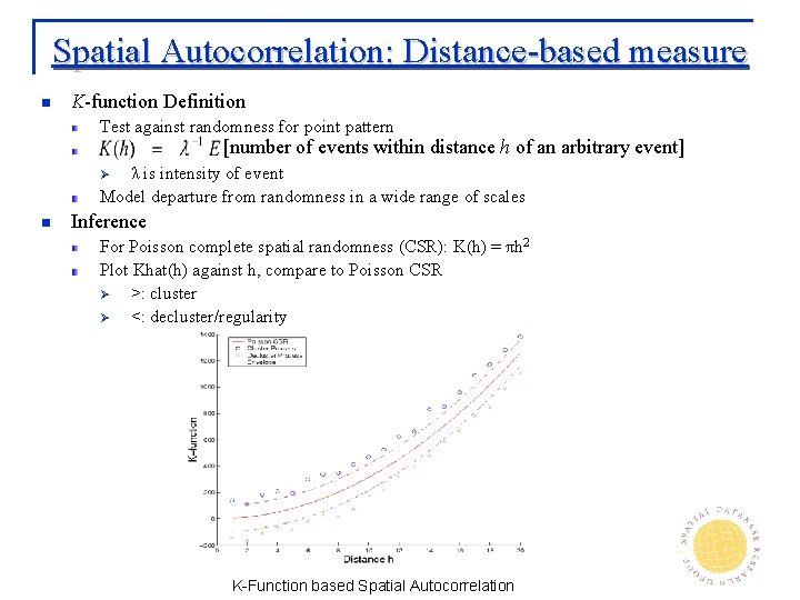
Spatial Autocorrelation: Distance-based measure n K-function Definition Test against randomness for point pattern [number of events within distance h of an arbitrary event] λ is intensity of event Model departure from randomness in a wide range of scales Ø n Inference For Poisson complete spatial randomness (CSR): K(h) = πh 2 Plot Khat(h) against h, compare to Poisson CSR Ø >: cluster Ø <: decluster/regularity K-Function based Spatial Autocorrelation

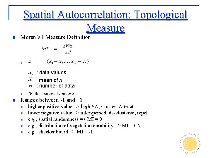
Spatial Autocorrelation: Topological Measure n Moran’s I Measure Definition : data values : mean of x : number of data W: the contiguity matrix n Ranges between -1 and +1 higher positive value => high SA, Cluster, Attract lower negative value => interspersed, de-clustered, repel e. g. , spatial randomness => MI = 0 e. g. , distribution of vegetation durability => MI = 0. 7 e. g. , checker board => MI = -1

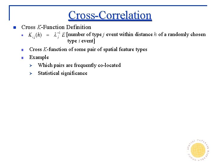
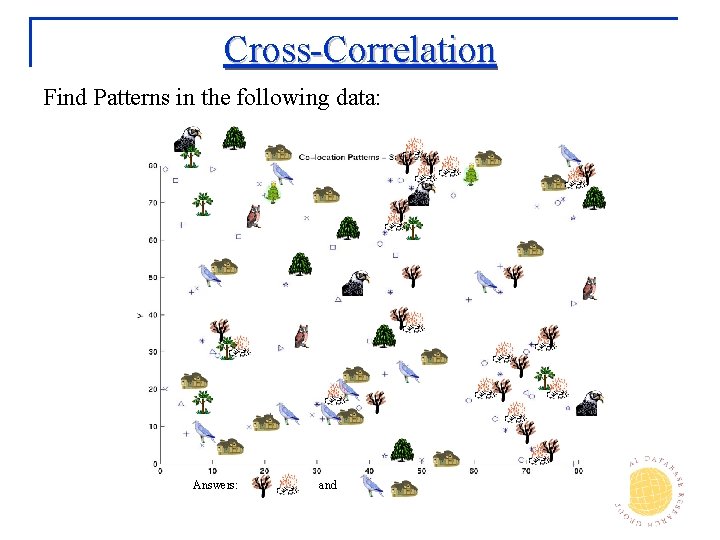
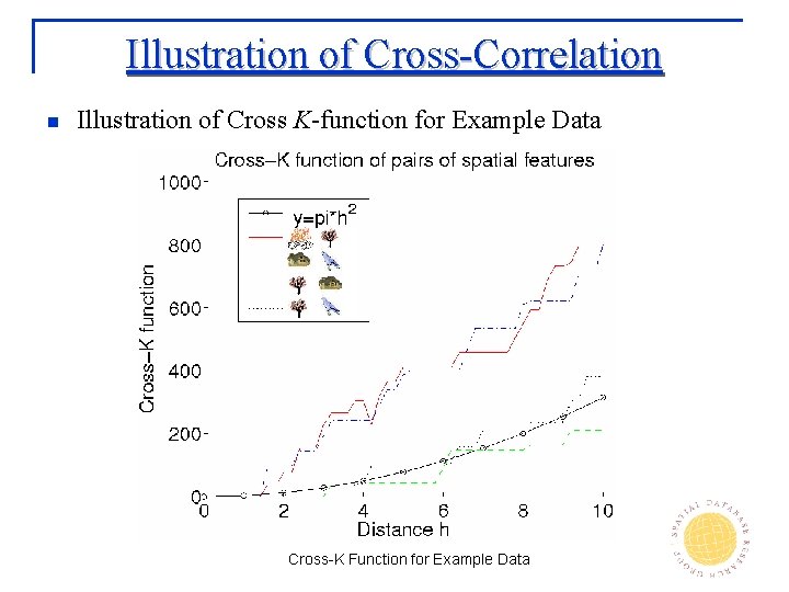
Cross-Correlation n Cross K-Function Definition [number of type j event within distance h of a randomly chosen type i event] Cross K-function of some pair of spatial feature types Example Ø Which pairs are frequently co-located Ø Statistical significance

Cross-Correlation Find Patterns in the following data: Answers: and

Illustration of Cross-Correlation n Illustration of Cross K-function for Example Data Cross-K Function for Example Data

Spatial Slicing n Spatial heterogeneity “Second law of geography” [M. Goodchild, UCGIS 2003] Global model might be inconsistent with regional models Ø spatial Simpson’s Paradox Global Model n Regional Models Spatial Slicing inputs can improve the effectiveness of SDM Slicing output can illustrate support regions of a pattern Ø e. g. , association rule with support map

Edge Effect n n Cropland on edges may not be classified as outliers No concept of spatial edges in classical data mining Korea Dataset, Courtesy: Architecture Technology Corporation

Research Challenges of Spatial Statistics n State-of-the-art of Spatial Statistics Point Process raster Vector Point √ Lattice Geostatistics √ √ Line Polygon √ √ graph Data Types and Statistical Models n n n Research Needs Correlating extended features: Ø e. g. road, river (line strings) Ø e. g. cropland (polygon), road, river Edge effect Relationship to classical statistics Ex. SVM with spatial basis function vs. SAR √

Overview ü ü Ø n n Input Statistical Foundation Output Computational Process Trends

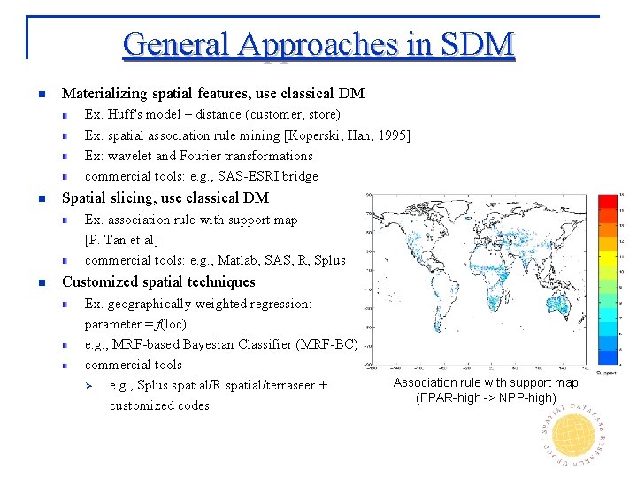
General Approaches in SDM n Materializing spatial features, use classical DM Ex. Huff's model – distance (customer, store) Ex. spatial association rule mining [Koperski, Han, 1995] Ex: wavelet and Fourier transformations commercial tools: e. g. , SAS-ESRI bridge n Spatial slicing, use classical DM Ex. association rule with support map [P. Tan et al] commercial tools: e. g. , Matlab, SAS, R, Splus n Customized spatial techniques Ex. geographically weighted regression: parameter = f(loc) e. g. , MRF-based Bayesian Classifier (MRF-BC) commercial tools Ø e. g. , Splus spatial/R spatial/terraseer + customized codes Association rule with support map (FPAR-high -> NPP-high)

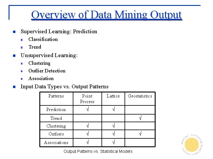
Overview of Data Mining Output n Supervised Learning: Prediction Classification Trend n Unsupervised Learning: Clustering Outlier Detection Association n Input Data Types vs. Output Patterns Point Process Lattice Prediction √ √ Geostatistics Trend √ Clustering √ √ Outliers √ √ Associations √ √ Output Patterns vs. Statistical Models √

Location Prediction Nest Locations Water Depth Vegetation Distance to Open Water

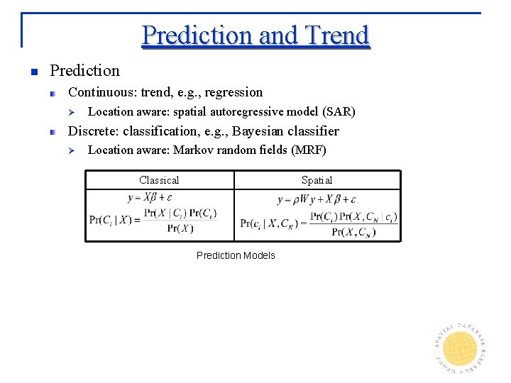
Prediction and Trend n Prediction Continuous: trend, e. g. , regression Ø Location aware: spatial autoregressive model (SAR) Discrete: classification, e. g. , Bayesian classifier Ø Location aware: Markov random fields (MRF) Classical Spatial Prediction Models

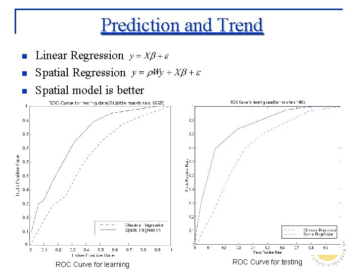
Prediction and Trend n n n Linear Regression Spatial model is better ROC Curve for learning ROC Curve for testing

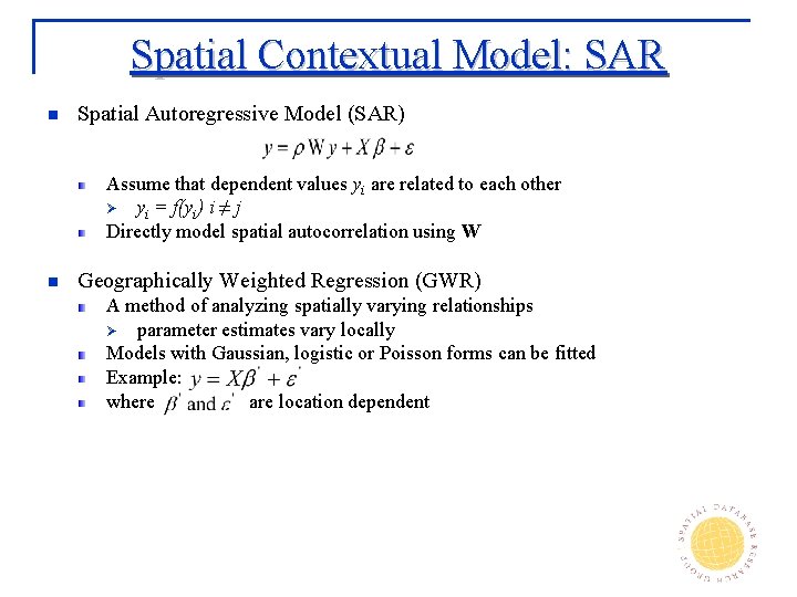
Spatial Contextual Model: SAR n Spatial Autoregressive Model (SAR) Assume that dependent values yi are related to each other Ø yi = f(yi) i ≠ j Directly model spatial autocorrelation using W n Geographically Weighted Regression (GWR) A method of analyzing spatially varying relationships Ø parameter estimates vary locally Models with Gaussian, logistic or Poisson forms can be fitted Example: where are location dependent

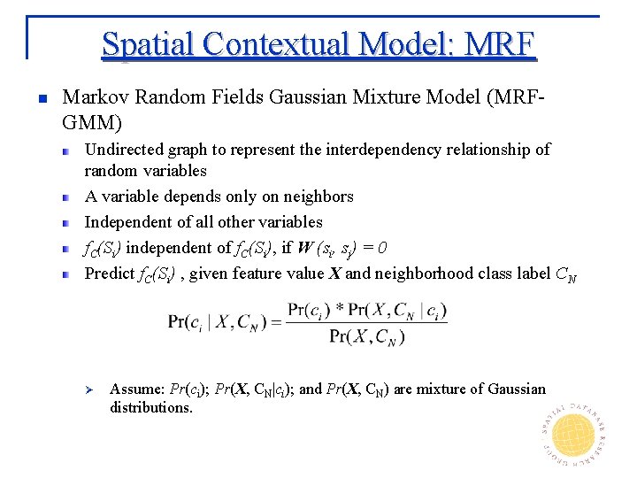
Spatial Contextual Model: MRF n Markov Random Fields Gaussian Mixture Model (MRFGMM) Undirected graph to represent the interdependency relationship of random variables A variable depends only on neighbors Independent of all other variables f. C(Si) independent of f. C(Si), if W (si, sj) = 0 Predict f. C(Si) , given feature value X and neighborhood class label CN Ø Assume: Pr(ci); Pr(X, CN|ci); and Pr(X, CN) are mixture of Gaussian distributions.

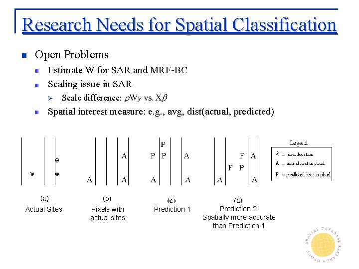
Research Needs for Spatial Classification n Open Problems Estimate W for SAR and MRF-BC Scaling issue in SAR Ø Scale difference: Spatial interest measure: e. g. , avg, dist(actual, predicted) Actual Sites Pixels with actual sites Prediction 1 Prediction 2. Spatially more accurate than Prediction 1

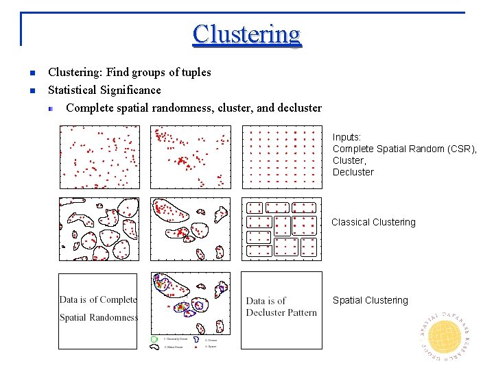
Clustering n n Clustering: Find groups of tuples Statistical Significance Complete spatial randomness, cluster, and decluster Inputs: Complete Spatial Random (CSR), Cluster, Decluster Classical Clustering Spatial Clustering

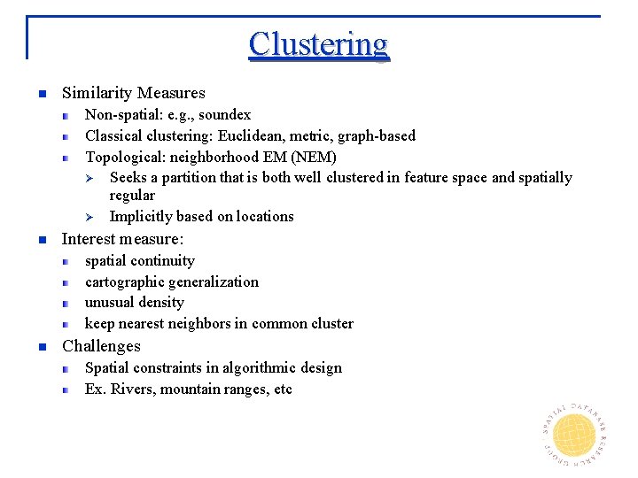
Clustering n Similarity Measures Non-spatial: e. g. , soundex Classical clustering: Euclidean, metric, graph-based Topological: neighborhood EM (NEM) Ø Seeks a partition that is both well clustered in feature space and spatially regular Ø Implicitly based on locations n Interest measure: spatial continuity cartographic generalization unusual density keep nearest neighbors in common cluster n Challenges Spatial constraints in algorithmic design Ex. Rivers, mountain ranges, etc

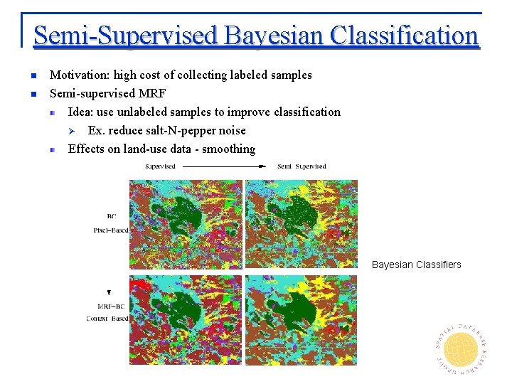
Semi-Supervised Bayesian Classification n n Motivation: high cost of collecting labeled samples Semi-supervised MRF Idea: use unlabeled samples to improve classification Ø Ex. reduce salt-N-pepper noise Effects on land-use data - smoothing Bayesian Classifiers

Outlier Detection n Spatial Outlier Detection Finding anomalous tuples Global and spatial outlier Detection Approaches Ø Graph-based outlier detection: variogram, Moran scatter plot Ø Quantitative outlier detection: scatter plot, and z-score n Location-awareness Outlier in Traffic Data

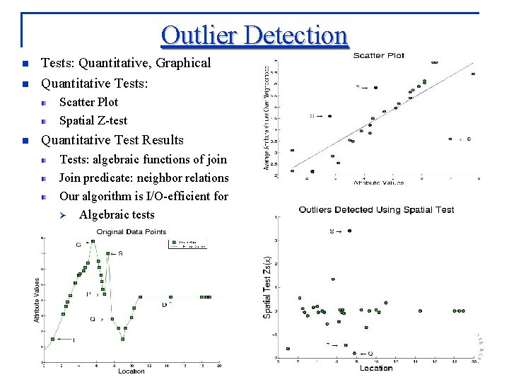
Outlier Detection n n Tests: Quantitative, Graphical Quantitative Tests: Scatter Plot Spatial Z-test n Quantitative Test Results Tests: algebraic functions of join Join predicate: neighbor relations Our algorithm is I/O-efficient for Ø Algebraic tests

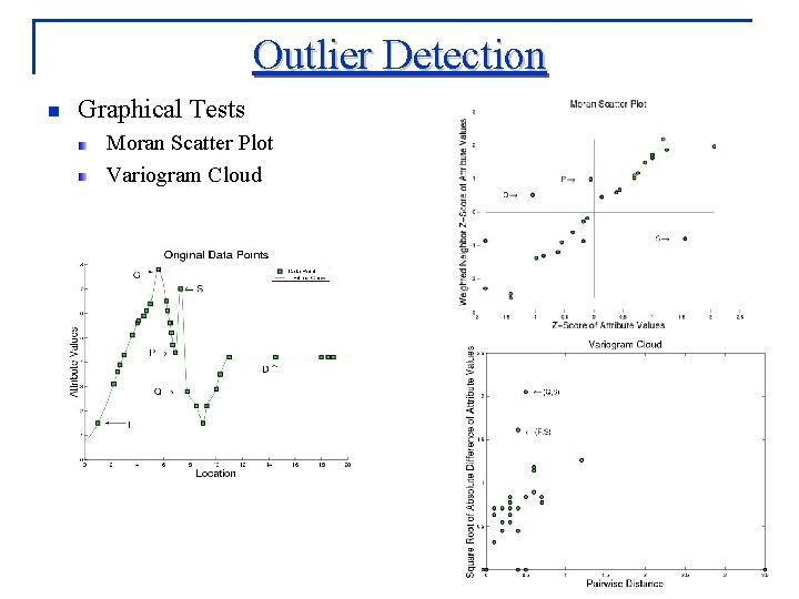
Outlier Detection n Graphical Tests Moran Scatter Plot Variogram Cloud

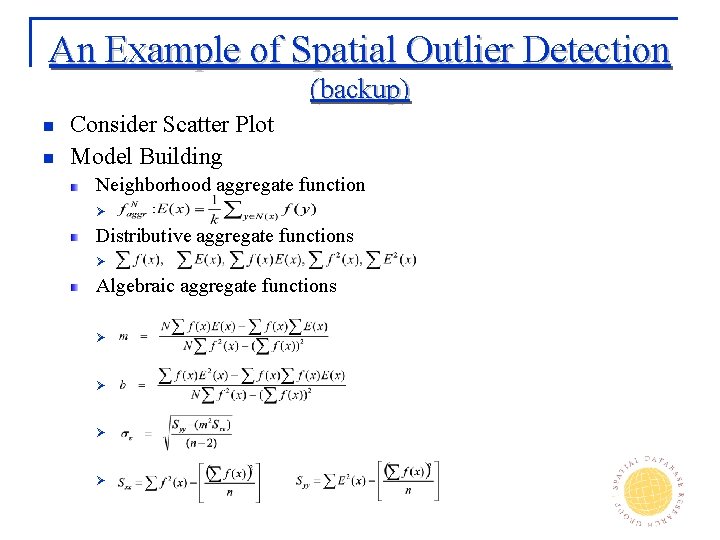
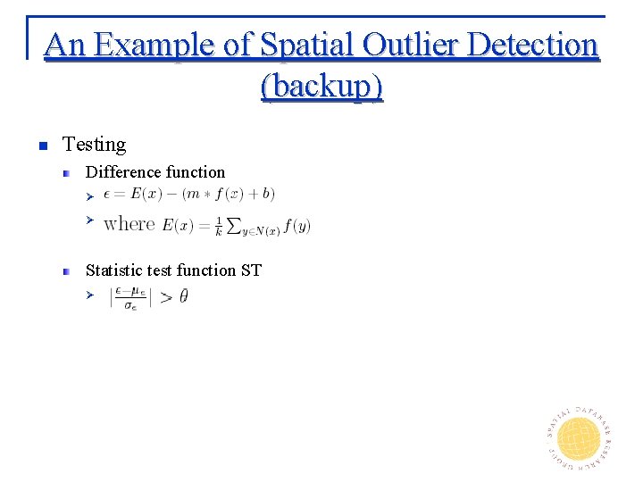
An Example of Spatial Outlier Detection (backup) n n Consider Scatter Plot Model Building Neighborhood aggregate function Ø Distributive aggregate functions Ø Algebraic aggregate functions Ø Ø

An Example of Spatial Outlier Detection (backup) n Testing Difference function Ø Ø Statistic test function ST Ø

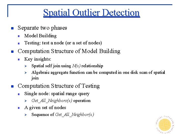
Spatial Outlier Detection n Separate two phases Model Building Testing: test a node (or a set of nodes) n Computation Structure of Model Building Key insights: Ø Ø n Spatial self join using N(x) relationship Algebraic aggregate function can be computed in one disk scan of spatial join Computation Structure of Testing Single node: spatial range query Ø Get_All_Neighbors(x) operation A given set of nodes Ø Sequence of Get_All_Neighbor(x)

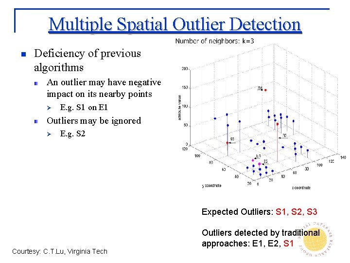
Multiple Spatial Outlier Detection n Deficiency of previous algorithms An outlier may have negative impact on its nearby points Ø E. g. S 1 on E 1 Outliers may be ignored Ø E. g. S 2 Expected Outliers: S 1, S 2, S 3 Courtesy: C. T. Lu, Virginia Tech Outliers detected by traditional approaches: E 1, E 2, S 1

Multiple Spatial Outlier Detection n Multiple Spatial Outlier Detection Iterative algorithm Ø Ø Detects one outlier in each iteration In successive iteration, substitute the attribute value of outlier detected in previous iteration with the average of its neighbors Median algorithm Ø Use Median, instead of Mean, to represent the average attribute value of neighbors

Research Needs in Spatial Outlier Detection n Multiple spatial outlier detection Eliminating the influence of neighboring outliers Incremental n Multi-attribute spatial outlier detection Use multiple attributes as features n n Design of spatial statistical tests Scale up for large data

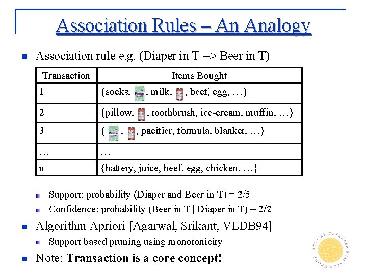
Association Rules – An Analogy n Association rule e. g. (Diaper in T => Beer in T) Transaction Items Bought 1 {socks, , milk, 2 {pillow, , toothbrush, ice-cream, muffin, …} 3 { … … n {battery, juice, beef, egg, chicken, …} , , beef, egg, …} , pacifier, formula, blanket, …} Support: probability (Diaper and Beer in T) = 2/5 Confidence: probability (Beer in T | Diaper in T) = 2/2 n Algorithm Apriori [Agarwal, Srikant, VLDB 94] Support based pruning using monotonicity n Note: Transaction is a core concept!

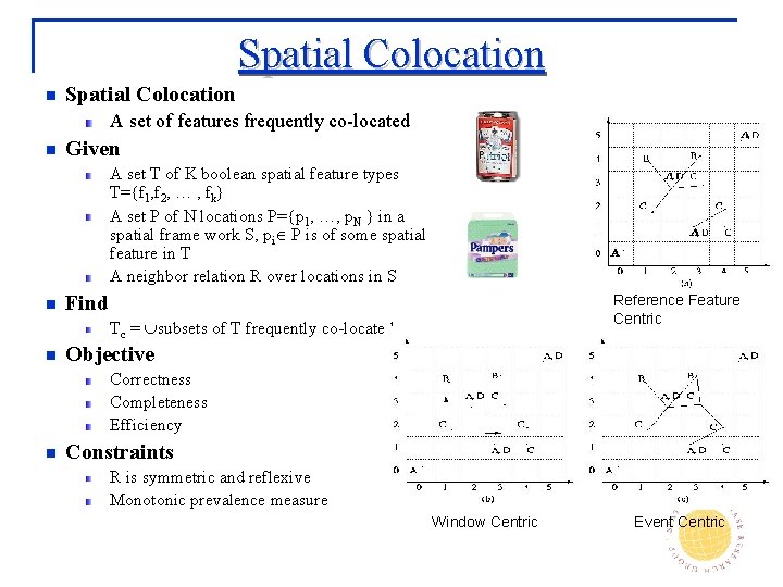
Spatial Colocation n Spatial Colocation A set of features frequently co-located n Given A set T of K boolean spatial feature types T={f 1, f 2, … , fk} A set P of N locations P={p 1, …, p. N } in a spatial frame work S, pi P is of some spatial feature in T A neighbor relation R over locations in S n Find Reference Feature Centric Tc = subsets of T frequently co-located n Objective Correctness Completeness Efficiency n Constraints R is symmetric and reflexive Monotonic prevalence measure Window Centric Event Centric

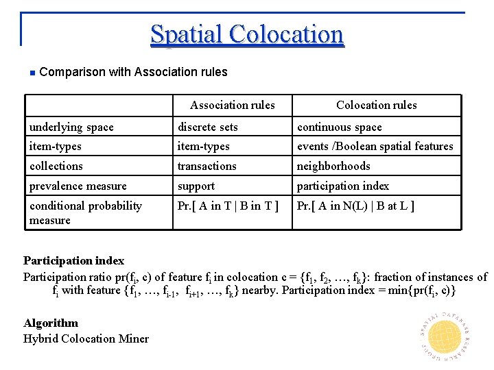
Spatial Colocation n Comparison with Association rules Colocation rules underlying space discrete sets continuous space item-types events /Boolean spatial features collections transactions neighborhoods prevalence measure support participation index conditional probability measure Pr. [ A in T | B in T ] Pr. [ A in N(L) | B at L ] Participation index Participation ratio pr(fi, c) of feature fi in colocation c = {f 1, f 2, …, fk}: fraction of instances of fi with feature {f 1, …, fi-1, fi+1, …, fk} nearby. Participation index = min{pr(fi, c)} Algorithm Hybrid Colocation Miner

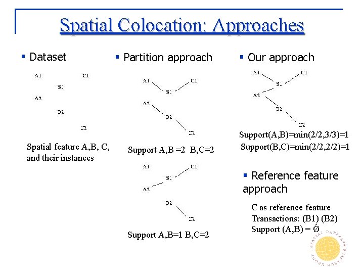
Spatial Colocation: Approaches § Dataset Spatial feature A, B, C, and their instances § Partition approach Support A, B =2 B, C=2 § Our approach Support(A, B)=min(2/2, 3/3)=1 Support(B, C)=min(2/2, 2/2)=1 § Reference feature approach Support A, B=1 B, C=2 C as reference feature Transactions: (B 1) (B 2) Support (A, B) = Ǿ

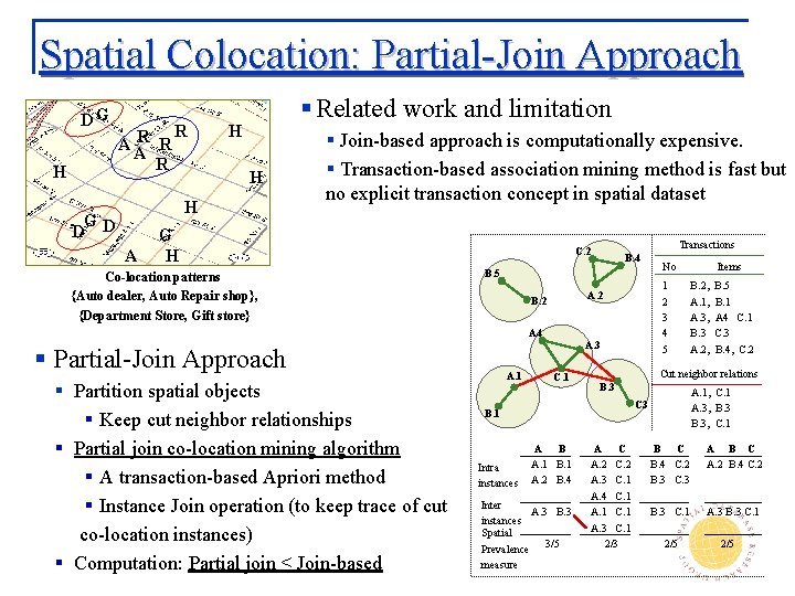
Spatial Colocation: Partial-Join Approach DG H R R AA R R § Related work and limitation H H H G D D A § Join-based approach is computationally expensive. § Transaction-based association mining method is fast but no explicit transaction concept in spatial dataset G H Co-location patterns {Auto dealer, Auto Repair shop}, {Department Store, Gift store} Transactions C. 2 B. 4 B. 5 1 2 3 4 5 A. 2 B. 2 A 4 A. 3 § Partial-Join Approach § Partition spatial objects § Keep cut neighbor relationships § Partial join co-location mining algorithm § A transaction-based Apriori method § Instance Join operation (to keep trace of cut co-location instances) § Computation: Partial join < Join-based A. 1 C. 1 Inter A. 3 B. 3 instances Spatial Prevalence 3/5 measure B. 2, A. 1, A. 3, B. 3 A. 2, B. 5 B. 1 A 4 C. 1 C. 3 B. 4, C. 2 A. 1, C. 1 A. 3, B. 3, C. 1 C 3 A B A. 1 B. 1 A. 2 B. 4 Items Cut neighbor relations B. 3 B. 1 Intra instances No A C A. 2 C. 2 A. 3 C. 1 A. 4 C. 1 A. 1 C. 1 A. 3 C. 1 2/3 B C B. 4 C. 2 B. 3 C. 3 A B C A. 2 B. 4 C. 2 B. 3 C. 1 A. 3 B. 3 C. 1 2/5

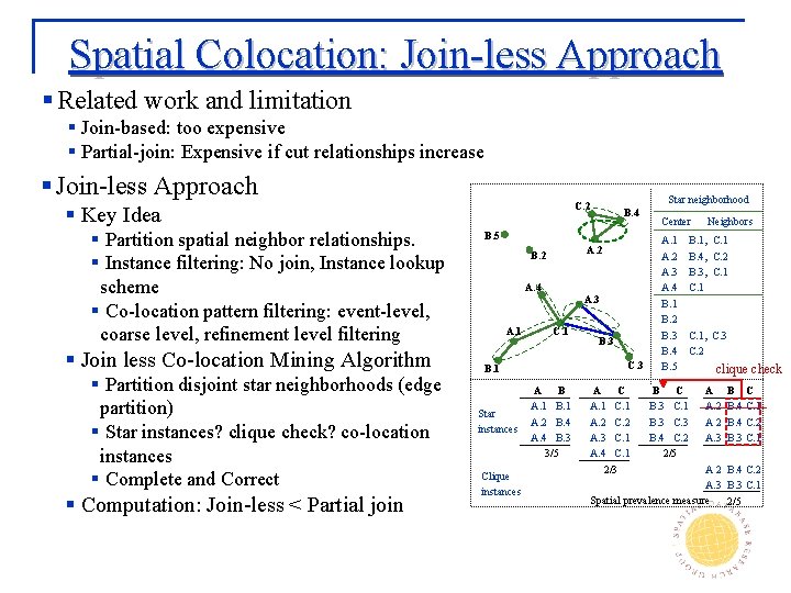
Spatial Colocation: Join-less Approach § Related work and limitation § Join-based: too expensive § Partial-join: Expensive if cut relationships increase § Join-less Approach § Key Idea § Partition spatial neighbor relationships. § Instance filtering: No join, Instance lookup scheme § Co-location pattern filtering: event-level, coarse level, refinement level filtering § Join less Co-location Mining Algorithm § Partition disjoint star neighborhoods (edge partition) § Star instances? clique check? co-location instances § Complete and Correct § Computation: Join-less < Partial join Star neighborhood C. 2 B. 4 B. 5 A. 2 B. 2 A. 4 A. 3 A. 1 C. 3 B. 1 Star instances Clique instances B. 3 A B A. 1 B. 1 A. 2 B. 4 A. 4 B. 3 3/5 A C A. 1 C. 1 A. 2 C. 2 A. 3 C. 1 A. 4 C. 1 2/3 Center Neighbors A. 1 B. 1, A. 2 B. 4, A. 3 B. 3, A. 4 C. 1 B. 2 B. 3 C. 1, B. 4 C. 2 B. 5 B C B. 3 C. 1 B. 3 C. 3 B. 4 C. 2 2/5 C. 1 C. 2 C. 1 C. 3 clique check A A. 2 A. 3 B C B. 4 C. 1 B. 4 C. 2 B. 3 C. 1 A 2 B. 4 C. 2 A. 3 B. 3 C. 1 Spatial prevalence measure 2/5

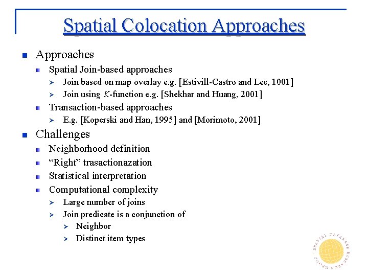
Spatial Colocation Approaches Spatial Join-based approaches Ø Ø Join based on map overlay e. g. [Estivill-Castro and Lee, 1001] Join using K-function e. g. [Shekhar and Huang, 2001] Transaction-based approaches Ø n E. g. [Koperski and Han, 1995] and [Morimoto, 2001] Challenges Neighborhood definition “Right” trasactionazation Statistical interpretation Computational complexity Ø Ø Large number of joins Join predicate is a conjunction of Ø Neighbor Ø Distinct item types

Overview ü ü ü Ø n Input Statistical Foundation Output Computational Process Trends

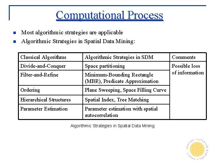
Computational Process n n Most algorithmic strategies are applicable Algorithmic Strategies in Spatial Data Mining: Classical Algorithms Algorithmic Strategies in SDM Comments Divide-and-Conquer Space partitioning Filter-and-Refine Minimum-Bounding Rectangle (MBR), Predicate Approximation Possible loss of information Ordering Plane Sweeping, Space Filling Curve Hierarchical Structures Spatial Index, Tree Matching Parameter Estimation Parameter estimation with spatial autocorrelation Algorithmic Strategies in Spatial Data Mining

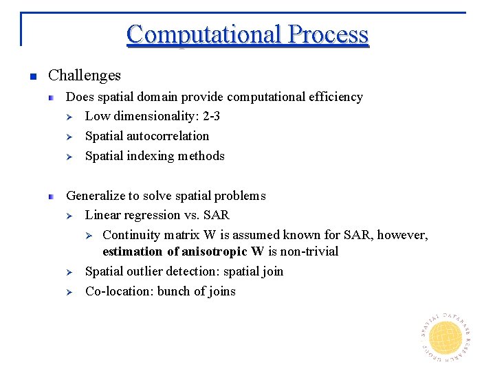
Computational Process n Challenges Does spatial domain provide computational efficiency Ø Low dimensionality: 2 -3 Ø Spatial autocorrelation Ø Spatial indexing methods Generalize to solve spatial problems Ø Linear regression vs. SAR Ø Continuity matrix W is assumed known for SAR, however, estimation of anisotropic W is non-trivial Ø Spatial outlier detection: spatial join Ø Co-location: bunch of joins

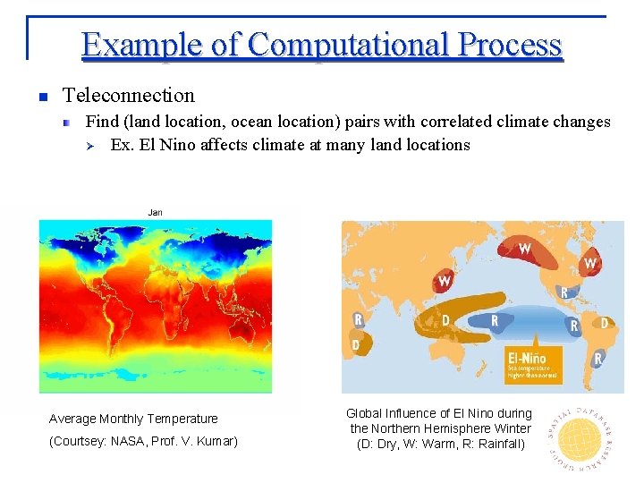
Example of Computational Process n Teleconnection Find (land location, ocean location) pairs with correlated climate changes Ø Ex. El Nino affects climate at many land locations Average Monthly Temperature (Courtsey: NASA, Prof. V. Kumar) Global Influence of El Nino during the Northern Hemisphere Winter (D: Dry, W: Warm, R: Rainfall)

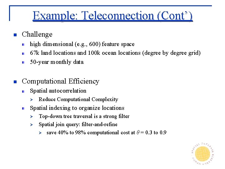
Example: Teleconnection (Cont’) n Challenge high dimensional (e. g. , 600) feature space 67 k land locations and 100 k ocean locations (degree by degree grid) 50 -year monthly data n Computational Efficiency Spatial autocorrelation Ø Reduce Computational Complexity Spatial indexing to organize locations Ø Ø Top-down tree traversal is a strong filter Spatial join query: filter-and-refine Ø save 40% to 98% computational cost at θ = 0. 3 to 0. 9

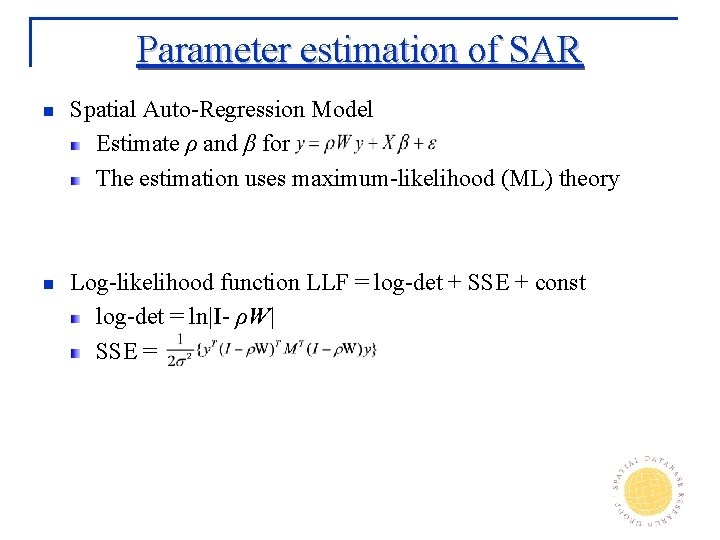
Parameter estimation of SAR n Spatial Auto-Regression Model Estimate ρ and β for The estimation uses maximum-likelihood (ML) theory n Log-likelihood function LLF = log-det + SSE + const log-det = ln|I- ρW| SSE =

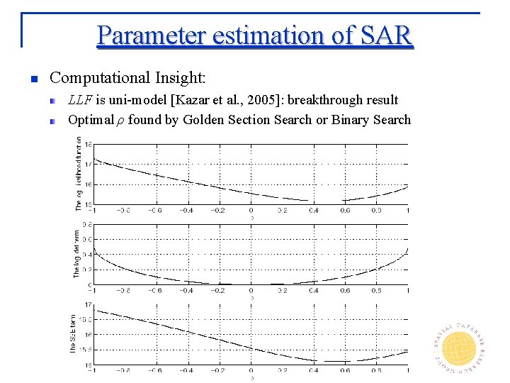
Parameter estimation of SAR n Computational Insight: LLF is uni-model [Kazar et al. , 2005]: breakthrough result Optimal ρ found by Golden Section Search or Binary Search

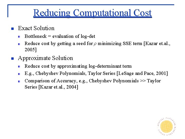
Reducing Computational Cost n Exact Solution Bottleneck = evaluation of log-det Reduce cost by getting a seed for ρ minimizing SSE term [Kazar et. al. , 2005] n Approximate Solution Reduce cost by approximating log-determinant term E. g. , Chebyshev Polynomials, Taylor Series [Le. Sage and Pace, 2001] Comparison of Accuracy, e. g. , Chebyshev Polynomials >> Taylor Series [Kazar et. al. , 2004]

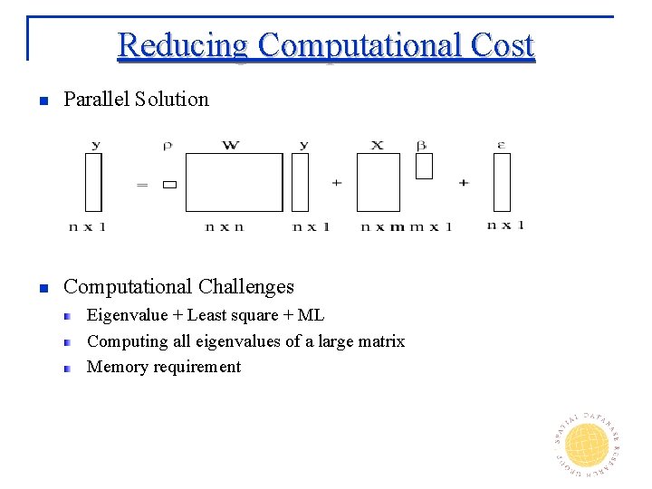
Reducing Computational Cost n Parallel Solution n Computational Challenges Eigenvalue + Least square + ML Computing all eigenvalues of a large matrix Memory requirement

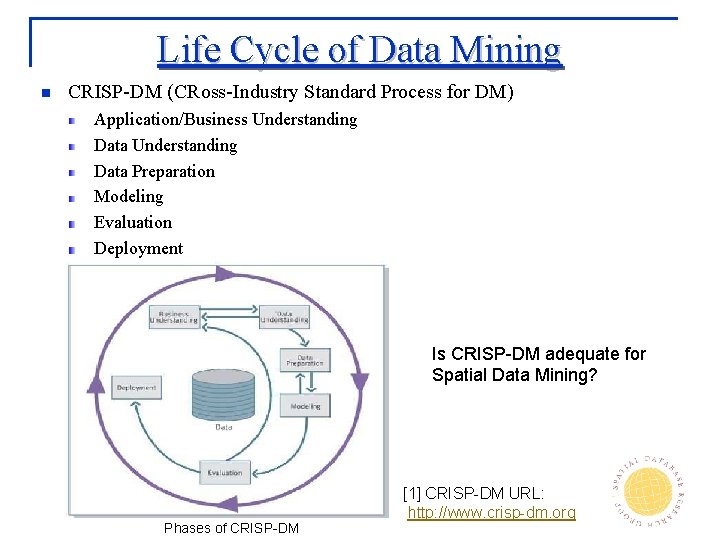
Life Cycle of Data Mining n CRISP-DM (CRoss-Industry Standard Process for DM) Application/Business Understanding Data Preparation Modeling Evaluation Deployment Is CRISP-DM adequate for Spatial Data Mining? Phases of CRISP-DM [1] CRISP-DM URL: http: //www. crisp-dm. org

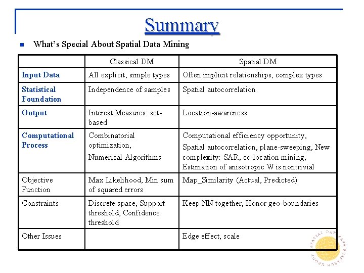
Summary n What’s Special About Spatial Data Mining Classical DM Spatial DM Input Data All explicit, simple types Often implicit relationships, complex types Statistical Foundation Independence of samples Spatial autocorrelation Output Interest Measures: setbased Location-awareness Computational Process Combinatorial optimization, Numerical Algorithms Computational efficiency opportunity, Spatial autocorrelation, plane-sweeping, New complexity: SAR, co-location mining, Estimation of anisotropic W is nontrivial Objective Function Max Likelihood, Min sum of squared errors Map_Similarity (Actual, Predicted) Constraints Discrete space, Support threshold, Confidence threshold Keep NN together, Honor geo-boundaries Other Issues Edge effect, scale

Overview ü ü Ø Input Statistical Foundation Output Computational Process Trends Ø Spatio-Temporal Data Mining

Trends: Spatio-Temporal Data Mining Ø § § Spatio-Temporal Data Spatio-Temporal Statistics Spatio-Temporal Patterns

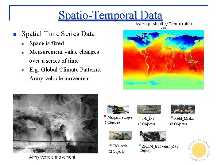
Spatio-Temporal Data Average Monthly Temperature n Spatial Time Series Data Space is fixed Measurement value changes over a series of time E. g. Global Climate Patterns, Army vehicle movement § Manpack stinger § M 2_IFV (1 Objects) § T 80_tank (2 Objects) Army vehicle movement (3 Objects) § Field_Marker (6 Objects) § BRDM_AT 5 (enemy) (1 Object)

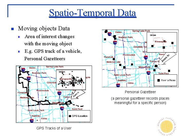
Spatio-Temporal Data n Moving objects Data Area of interest changes with the moving object E. g. GPS track of a vehicle, Personal Gazetteers Personal Gazetteer (a personal gazetteer records places meaningful for a specific person) GPS Tracks of a User

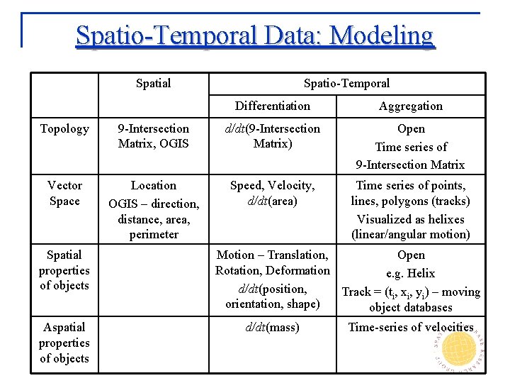
Spatio-Temporal Data: Modeling Spatial Spatio-Temporal Differentiation Aggregation Topology 9 -Intersection Matrix, OGIS d/dt(9 -Intersection Matrix) Open Time series of 9 -Intersection Matrix Vector Space Location OGIS – direction, distance, area, perimeter Speed, Velocity, d/dt(area) Time series of points, lines, polygons (tracks) Visualized as helixes (linear/angular motion) Spatial properties of objects Aspatial properties of objects Motion – Translation, Open Rotation, Deformation e. g. Helix d/dt(position, Track = (ti, xi, yi) – moving orientation, shape) object databases d/dt(mass) Time-series of velocities

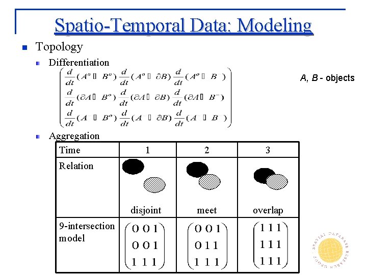
Spatio-Temporal Data: Modeling n Topology Differentiation A, B - objects Aggregation Time 1 2 3 disjoint meet overlap Relation 9 -intersection model

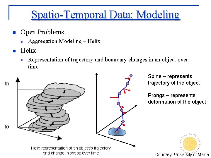
Spatio-Temporal Data: Modeling n Open Problems Aggregation Modeling – Helix n Helix Representation of trajectory and boundary changes in an object over time Spine – represents trajectory of the object Prongs – represents deformation of the object Helix representation of an object’s trajectory and change in shape over time Courtesy: University of Maine

Trends: Spatio-Temporal Data Mining § Ø § Spatio-Temporal Data Spatio-Temporal Statistics Spatio-Temporal Patterns

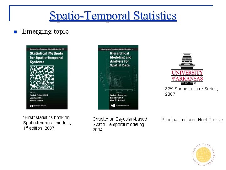
Spatio-Temporal Statistics n Emerging topic 32 nd Spring Lecture Series, 2007 “First” statistics book on Spatio-temporal models, 1 st edition, 2007 Chapter on Bayesian-based Spatio-Temporal modeling, 2004 Principal Lecturer: Noel Cressie

Trends: Spatio-Temporal Data Mining § § Ø Spatio-Temporal Data Spatio-Temporal Statistics Spatio-Temporal Patterns

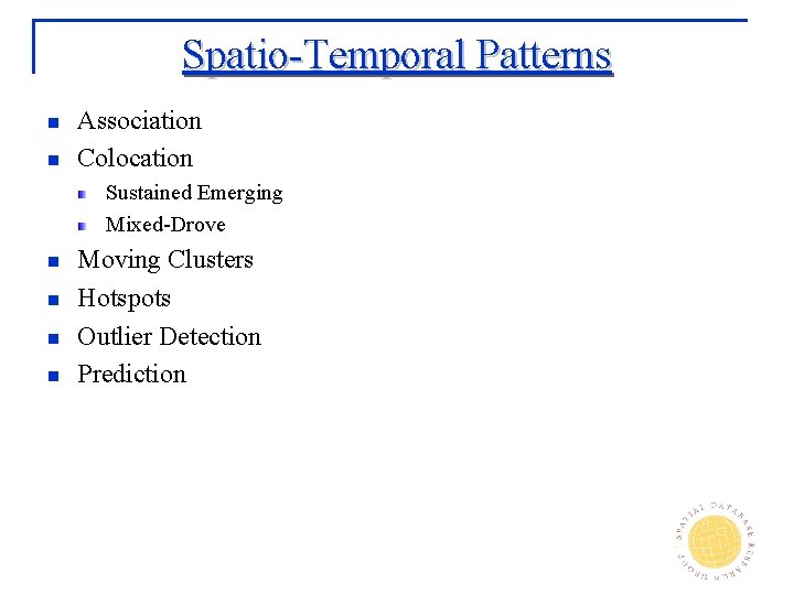
Spatio-Temporal Patterns n n Association Colocation Sustained Emerging Mixed-Drove n n Moving Clusters Hotspots Outlier Detection Prediction

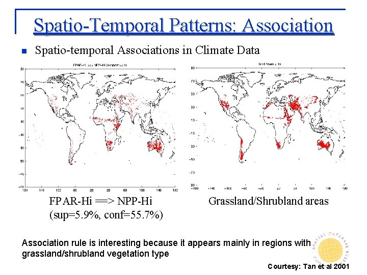
Spatio-Temporal Patterns: Association n Spatio-temporal Associations in Climate Data FPAR-Hi ==> NPP-Hi (sup=5. 9%, conf=55. 7%) Grassland/Shrubland areas Association rule is interesting because it appears mainly in regions with grassland/shrubland vegetation type Courtesy: Tan et al 2001

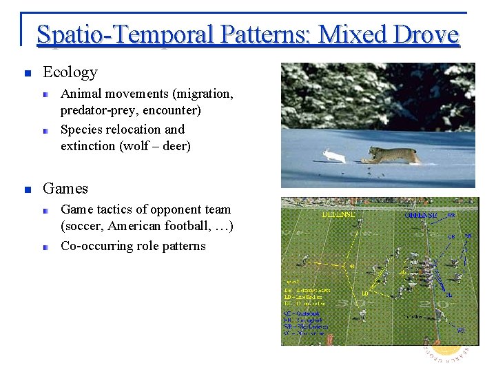
Spatio-Temporal Patterns: Mixed Drove n Ecology Animal movements (migration, predator-prey, encounter) Species relocation and extinction (wolf – deer) n Games Game tactics of opponent team (soccer, American football, …) Co-occurring role patterns

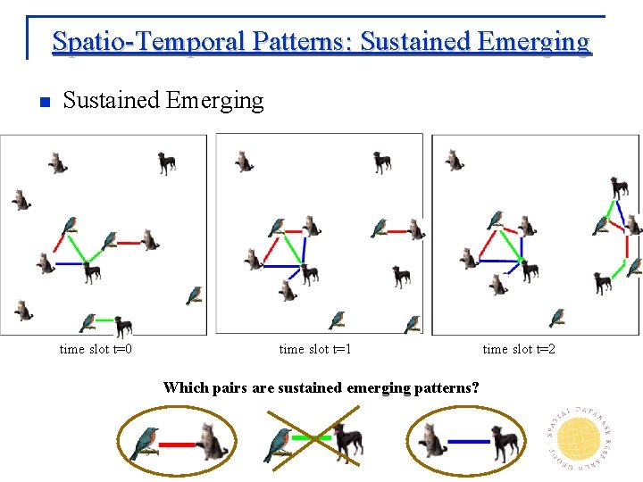
Spatio-Temporal Patterns: Sustained Emerging n Sustained Emerging time slot t=0 time slot t=1 Which pairs are sustained emerging patterns? time slot t=2

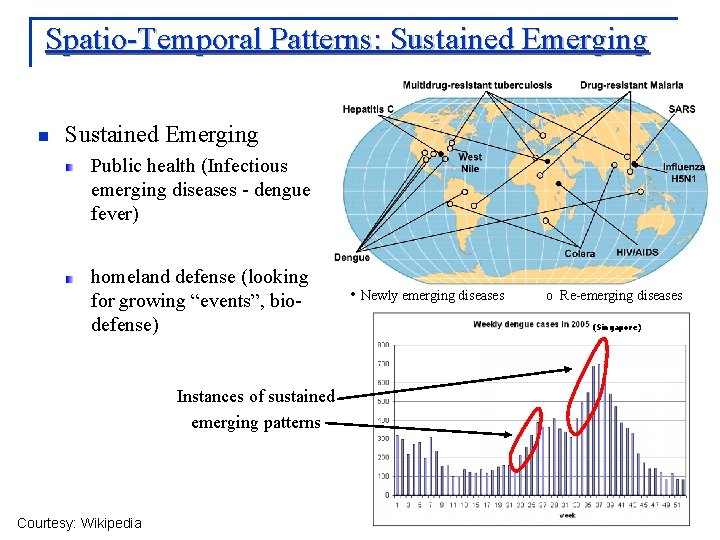
Spatio-Temporal Patterns: Sustained Emerging n Sustained Emerging Public health (Infectious emerging diseases - dengue fever) homeland defense (looking for growing “events”, biodefense) Instances of sustained emerging patterns Courtesy: Wikipedia • Newly emerging diseases o Re-emerging diseases (Singapore)

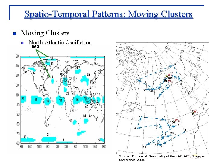
Spatio-Temporal Patterns: Moving Clusters n Moving Clusters North Atlantic Oscillation Source: Portis et al, Seasonality of the NAO, AGU Chapman Conference, 2000.

Spatio-Temporal Patterns: Mixed Drove n Flock Pattern Mining n Flock Pattern [Gudmundsson 05] Each time step treated separately Time Patterns 1 -10 3 -9 3 -9 AB AC BC ABC 7 7 AD BD CD ABCB • Significant Flock Patterns Interest Measure (threshold 0. 5) (A B) (A C) (B C) (A B C) others 1 0. 7 below threshold

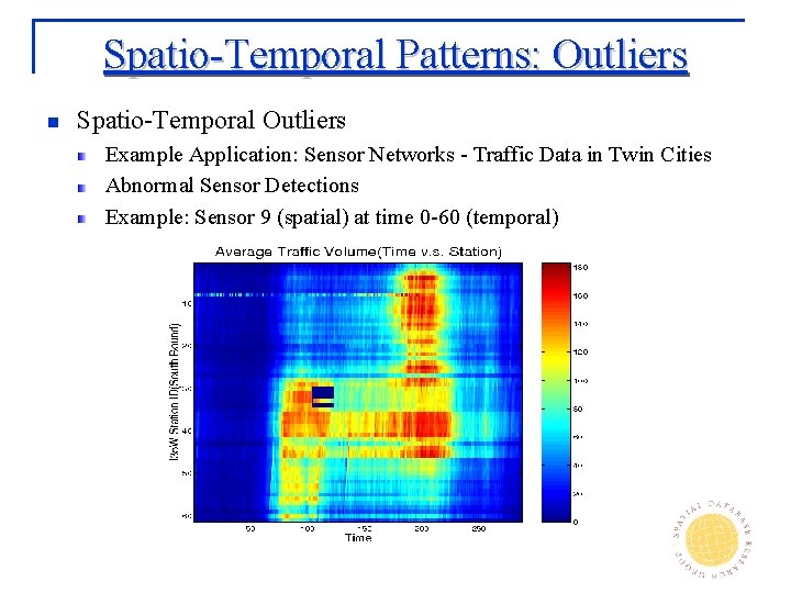
Spatio-Temporal Patterns: Outliers n Spatio-Temporal Outliers Example Application: Sensor Networks - Traffic Data in Twin Cities Abnormal Sensor Detections Example: Sensor 9 (spatial) at time 0 -60 (temporal)

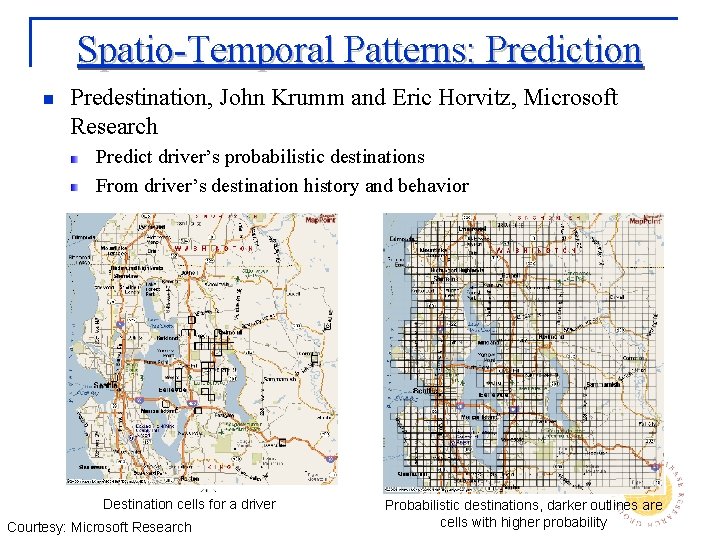
Spatio-Temporal Patterns: Prediction n Predestination, John Krumm and Eric Horvitz, Microsoft Research Predict driver’s probabilistic destinations From driver’s destination history and behavior Destination cells for a driver Courtesy: Microsoft Research Probabilistic destinations, darker outlines are cells with higher probability

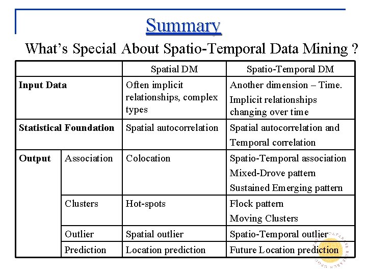
Summary What’s Special About Spatio-Temporal Data Mining ? Spatial DM Spatio-Temporal DM Input Data Often implicit relationships, complex types Another dimension – Time. Implicit relationships changing over time Statistical Foundation Spatial autocorrelation and Temporal correlation Output Association Colocation Spatio-Temporal association Mixed-Drove pattern Sustained Emerging pattern Clusters Hot-spots Flock pattern Moving Clusters Outlier Spatial outlier Spatio-Temporal outlier Prediction Location prediction Future Location prediction

Book http: //www. spatial. cs. umn. edu

References n N. Cressie, Statistics for Spatial Data, John Wiley and Sons, 1991 n M. Degroot and M. Schervish, Probability and Statistics (Third Ed. ), Addison Wesley, 2002 n A. Fotheringham, C. Brunsdon, and M. Charlton, Geographically Weighted Regression : The Analysis of Spatially Varying Relationships, John Wiley, 2002 n M. Goodchild, Spatial Analysis and GIS, 2001 ESRI User Conference Pre-Conference Seminar n R. Hanning, Spatial Data Analysis : Theory and Practice, Cambridge University Press, 2003 n Hastie, R. Tibshirani, and J. Friedman, The Elements of Statistical Learning, Springer-Verlag, 2001 n D. Huff, A Probabilistic Analysis of Shopping Center Trade Areas, Lan Economics, 1963 n B. M. Kazar, S. Shekhar, D. J. Lilja, R. R. Vatsavai, R. K. Pace, Comparing Exact and Approximate Spatial Auto-Regression Model Solutions for Spatial Data Analysis, GIScience 2004

References n K. Kopperski and J. Han, Discovery of Spatial Association Rules in Geographic Information Database, SSTD, 1995 n K. Kopperski, J. Adhikary, and J. Han, Spatial Data Mining: Progress and Challenges, DMKD, 1996 n J. Le. Sage and R. K. Pace, Spatial Dependence in Data Mining, in Data Mining for Scientific and Engineering Applications, R. L. Grossman, C. Kamath, P. Kegelmeyer, V. Kumar, and R. R. Namburu (eds. ), Kluwer Academic Publishing, p. 439 -460, 2001. n H. Miller and J. Han(eds), Geographic Data Mining and Knowledge Discovery, Taylor and Francis, 2001 n J. Roddick, K. Hornsby and M. Spiliopoulou, Yet Another Bibliography of Temporal, Spatial Spatio-temporal Data Mining Research, KDD Workshop, 2001 n S. Shekhar, C. T. Lu, and P. Zhang, A Unified Approach to Detecting Spatial Outliers, Geo. Informatica, 7(2), Kluwer Academic Publishers, 2003

References n S. Shekhar and S. Chawla, Spatial Databases: A Tour, Prentice Hall, 2003 n S. Shekhar, P. Schrater, R. Vatsavai, W. Wu, and S. Chawla, Spatial Contextual Classification and Prediction Models for Mining Geospatial Data, IEEE Transactions on Multimedia (special issue on Multimedia Databases), 2002 n S. Shekhar and Y. Huang, Discovering Spatial Co-location Patterns: A Summary of Results, SSTD, 2001 n P. Tan and M. Steinbach and V. Kumar and C. Potter and S. Klooster and A. Torregrosa, Finding Spatio-Temporal Patterns in Earth Science Data, KDD Workshop on Temporal Data Mining, 2001 n W. Tobler, A Computer Movie Simulating Urban Growth of Detroit Region, Economic Geography, 46: 236 -240, 1970 n P. Zhang, Y. Huang, S. Shekhar, and V. Kumar, Exploiting Spatial Autocorrelation to Efficiently Process Correlation-Based Similarity Queries, SSTD, 2003 n P. Zhang, M. Steinbach, V. Kumar, S. Shekhar, P. Tan, S. Klooster, C. Potter, Discovery of Patterns of Earth Science Data Using Data Mining, to appear in Next Generation of Data Mining Applications, edited by Mehmed M. Kantardzic and Jozef Zurada, IEEE Press, 2005

References n K. Eickhorst, A. Croitoru, P. Agouris & A. Stefanidis (2004): Spatiotemporal Helixes for Environmental Data Modeling, IEEE Comp. SAC, Hong Kong, Vol. 2, pp. 138 -141. n H. Cao, N. Mamoulis, and D. W. Cheung, "Discovery of Periodic Patterns in Spatiotemporal Sequences, " IEEE Transactions on Knowledge and Data Engineering (TKDE), to appear. n Marios Hadjieletheriou, George Kollios, Petko Bakalov, and Vassilis Tsotras. Complex Spatio -Temporal Pattern Queries. Proc. of the 31 st International Conference on Very Large Data Bases (VLDB), Trondheim, Norway, August 2005. n Nikos Mamoulis, Huping Cao, George Kollios, Marios Hadjieleftheriou, Yufei Tao, and David Cheung. Mining, Indexing, and Querying Historical Spatio-Temporal Data. Proceedings of the 10 th ACM International Conference on Knowledge Discovery and Data Mining (SIGKDD), Seattle, WA, August 2004. n Sanjay Chawla, Florian Verhein. Mining Spatio-Temporal Association Rules, Sources, Sinks, Stationary Regions and Thourough. Fares in Object Mobility Databases" Proc. of 11 th International Conference on Database Systems for Advanced Applications (DASFAA'06) n B. Arunasalam, S. Chawla and P. Sun, Striking Two Birds With One Stone: Simultaneous Mining of Positive and Negative Spatial Patterns, In Proceedings of the Fifth SIAM International Conference on Data Mining, Newport Beach, CA, 2005.

Google Earth video…focusing Metrodome