SPATIAL DATA ANALYSIS Tony E Smith University of

SPATIAL DATA ANALYSIS Tony E. Smith University of Pennsylvania • Point Pattern Analysis • Spatial Regression Analysis • Continuous Pattern Analysis

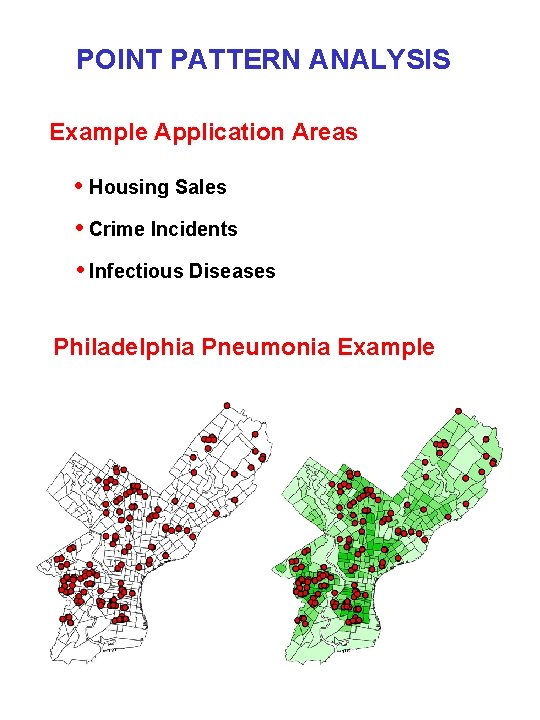
POINT PATTERN ANALYSIS Example Application Areas • Housing Sales • Crime Incidents • Infectious Diseases Philadelphia Pneumonia Example

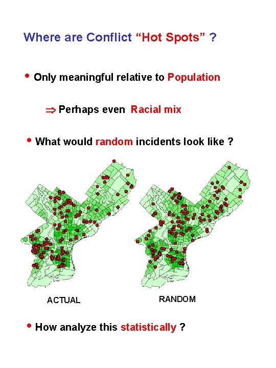
Where are Conflict “Hot Spots” ? • Only meaningful relative to Population Perhaps even Racial mix • What would random incidents look like ? ACTUAL RANDOM • How analyze this statistically ?

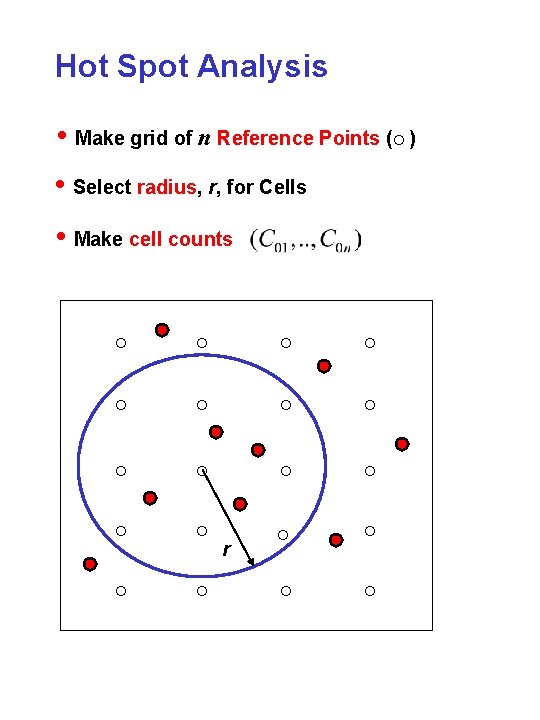
Hot Spot Analysis • Make grid of n Reference Points (° ) • Select radius, r, for Cells • Make cell counts ° ° ° ° ° r

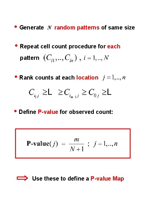
• Generate N random patterns of same size • Repeat cell count procedure for each pattern • Rank counts at each location • Define P-value for observed count: Use these to define a P-value Map

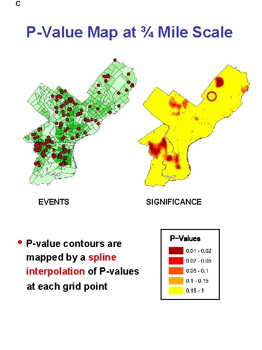
P-Value Map at ¾ Mile Scale EVENTS • P-value contours are mapped by a spline interpolation of P-values at each grid point SIGNIFICANCE P-Values

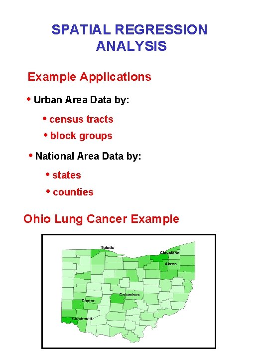
SPATIAL REGRESSION ANALYSIS Example Applications • Urban Area Data by: • census tracts • block groups • National Area Data by: • states • counties Ohio Lung Cancer Example

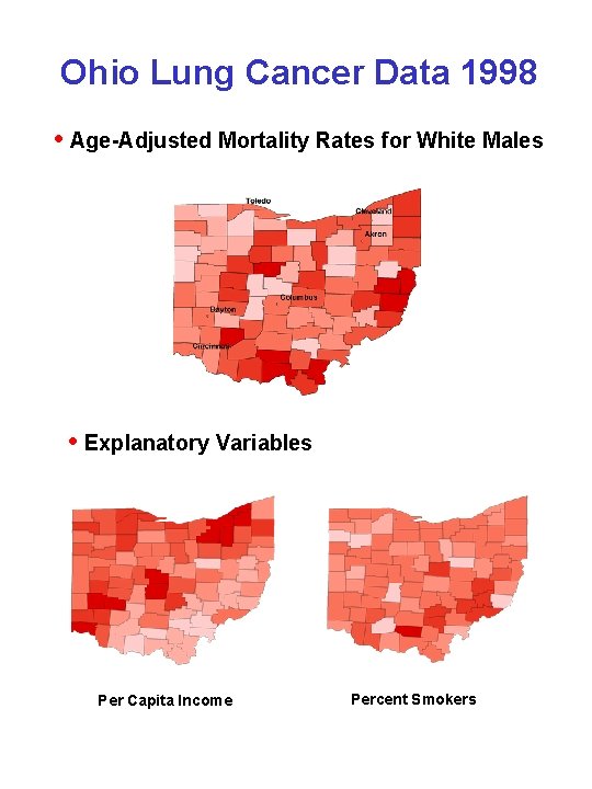
Ohio Lung Cancer Data 1998 • Age-Adjusted Mortality Rates for White Males • Explanatory Variables Per Capita Income Percent Smokers

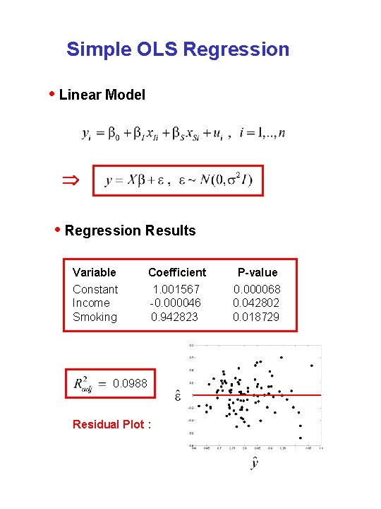
Simple OLS Regression • Linear Model • Regression Results Variable Constant Income Smoking Coefficient 1. 001567 -0. 000046 0. 942823 0. 0988 Residual Plot : P-value 0. 000068 0. 042802 0. 018729

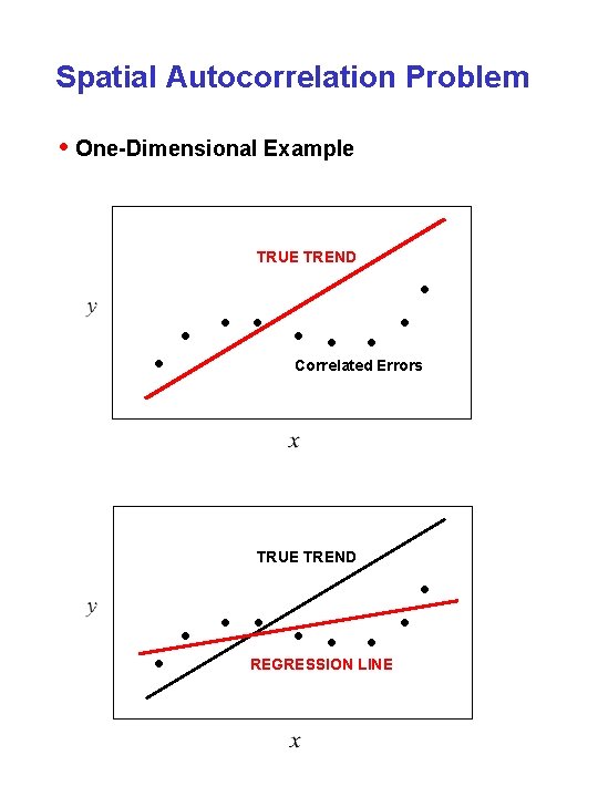
Spatial Autocorrelation Problem • One-Dimensional Example TRUE TREND • • • Correlated Errors TRUE TREND • • REGRESSION LINE •

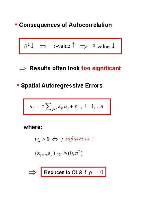
• Consequences of Autocorrelation Results often look too significant • Spatial Autoregressive Errors where: j influences i iid Reduces to OLS if

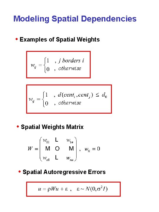
Modeling Spatial Dependencies • Examples of Spatial Weights , otherwise • Spatial Weights Matrix • Spatial Autoregressive Errors

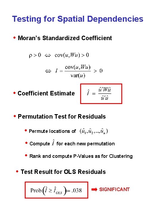
Testing for Spatial Dependencies • Moran’s Standardized Coefficient • Coefficient Estimate • Permutation Test for Residuals • Permute locations of • Compute for each new permutation • Rank and compute P-Values as for Clustering • Test Result for OLS Residuals SIGNIFICANT

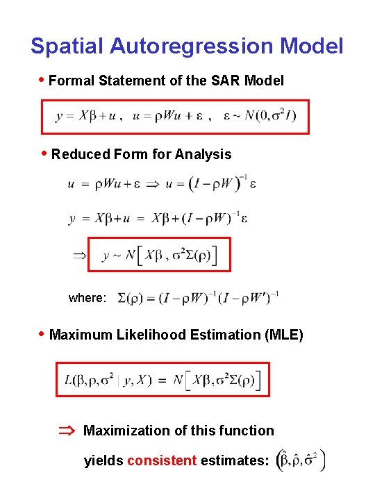
Spatial Autoregression Model • Formal Statement of the SAR Model • Reduced Form for Analysis where: • Maximum Likelihood Estimation (MLE) Maximization of this function yields consistent estimates:

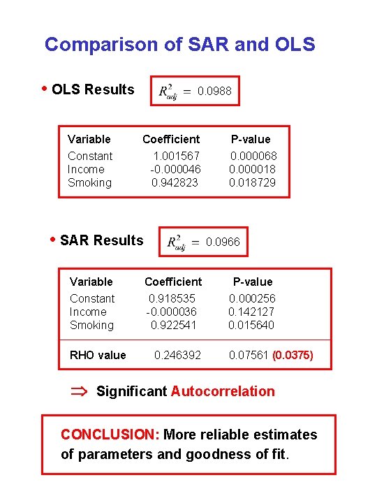
Comparison of SAR and OLS • OLS Results 0. 0988 Variable Coefficient Constant Income Smoking 1. 001567 -0. 000046 0. 942823 • SAR Results P-value 0. 000068 0. 000018 0. 018729 0. 0966 Variable Coefficient P-value Constant Income Smoking 0. 918535 -0. 000036 0. 922541 0. 000256 0. 142127 0. 015640 RHO value 0. 246392 0. 07561 (0. 0375) Significant Autocorrelation CONCLUSION: More reliable estimates of parameters and goodness of fit.

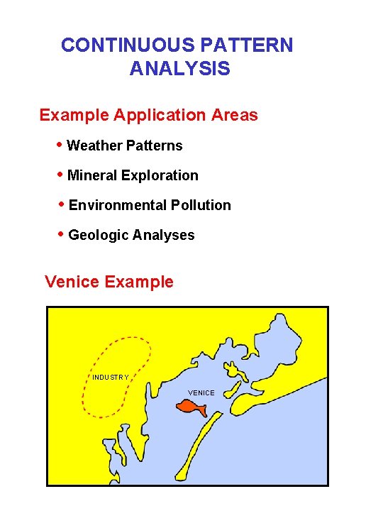
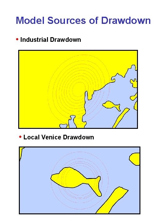
CONTINUOUS PATTERN ANALYSIS Example Application Areas • Weather Patterns • Mineral Exploration • Environmental Pollution • Geologic Analyses Venice Example INDUSTRY VENICE

Model Sources of Drawdown • Industrial Drawdown • Local Venice Drawdown

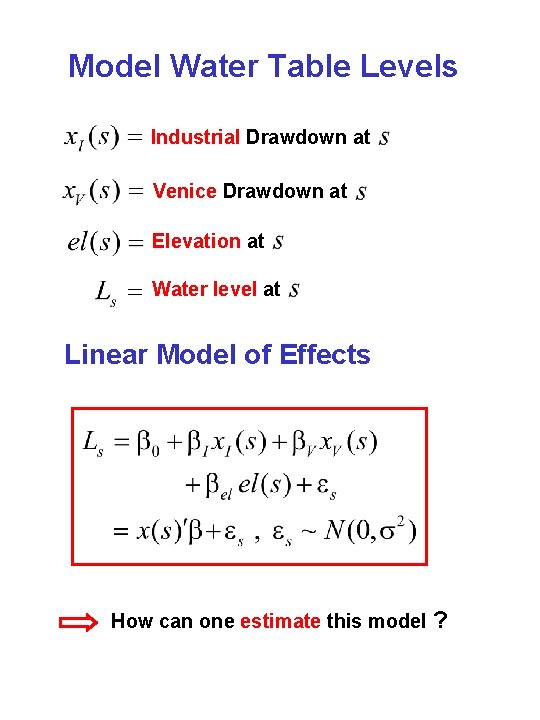
Model Water Table Levels Industrial Drawdown at Venice Drawdown at Elevation at Water level at Linear Model of Effects How can one estimate this model ?

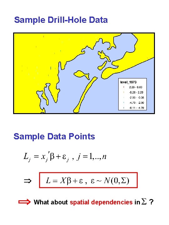
Sample Drill-Hole Data Sample Data Points What about spatial dependencies in ?

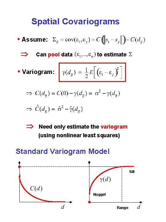
Spatial Covariograms • Assume: Can pool data to estimate • Variogram: Need only estimate the variogram (using nonlinear least squares) Standard Variogram Model Sill Nugget Range

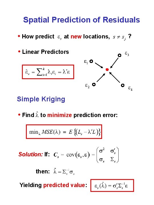
Spatial Prediction of Residuals • How predict at new locations, • Linear Predictors Simple Kriging • Find to minimize prediction error: Solution: If: then: Yielding predicted value: ?

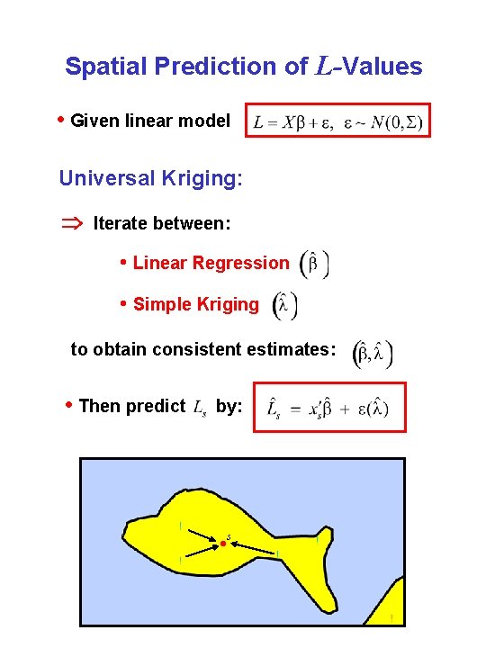
Spatial Prediction of L-Values • Given linear model Universal Kriging: Iterate between: • Linear Regression • Simple Kriging to obtain consistent estimates: • Then predict by: • s •

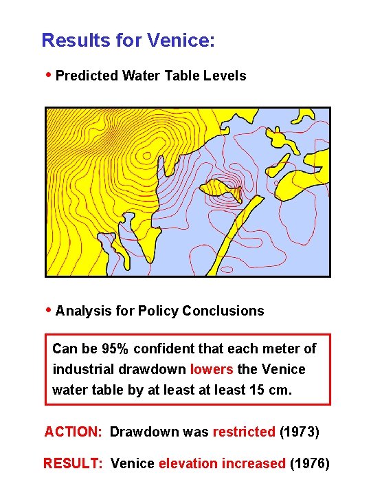
Results for Venice: • Predicted Water Table Levels • Analysis for Policy Conclusions Can be 95% confident that each meter of industrial drawdown lowers the Venice water table by at least 15 cm. ACTION: Drawdown was restricted (1973) RESULT: Venice elevation increased (1976)