Spatial Data Analysis Surfaces ModelDriven Approaches n Model

Spatial Data Analysis: Surfaces

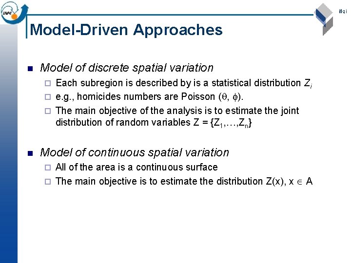
Model-Driven Approaches n Model of discrete spatial variation Each subregion is described by is a statistical distribution Zi ¨ e. g. , homicides numbers are Poisson ( , ). ¨ The main objective of the analysis is to estimate the joint distribution of random variables Z = {Z 1, …, Zn} ¨ n Model of continuous spatial variation All of the area is a continuous surface ¨ The main objective is to estimate the distribution Z(x), x A ¨

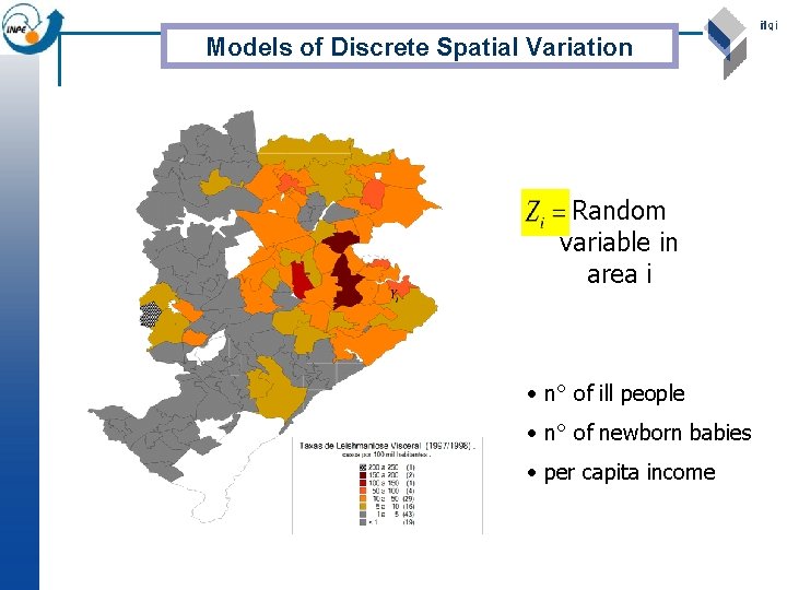
Models of Discrete Spatial Variation Random variable in area i • n° of ill people • n° of newborn babies • per capita income

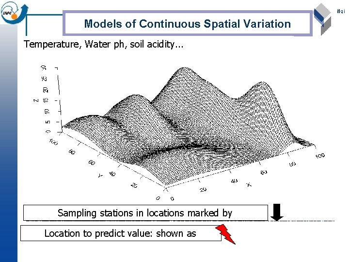
Models of Continuous Spatial Variation Temperature, Water ph, soil acidity. . . Sampling stations in locations marked by Location to predict value: shown as

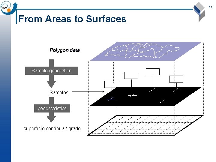
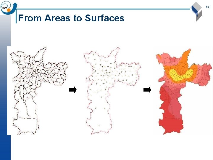
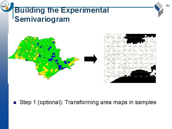
From Areas to Surfaces Polygon data Sample generation X, Y, Z Samples geoestatistics superfície contínua / grade X, Y, Z

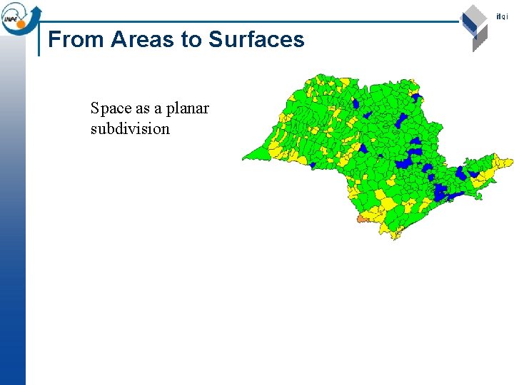
From Areas to Surfaces Space as a planar subdivision

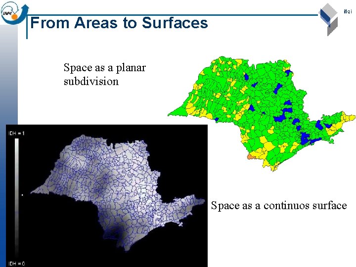
From Areas to Surfaces Space as a planar subdivision Space as a continuos surface

From Areas to Surfaces

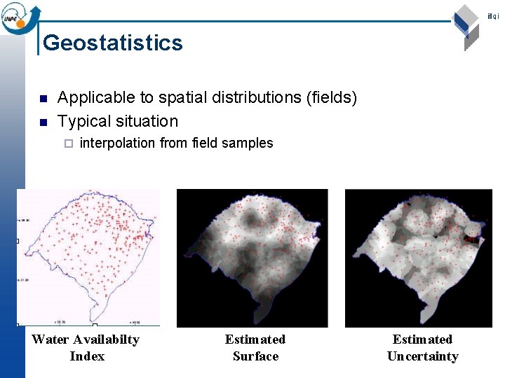
Geostatistics n n Applicable to spatial distributions (fields) Typical situation ¨ interpolation from field samples Water Availabilty Index Estimated Surface Estimated Uncertainty

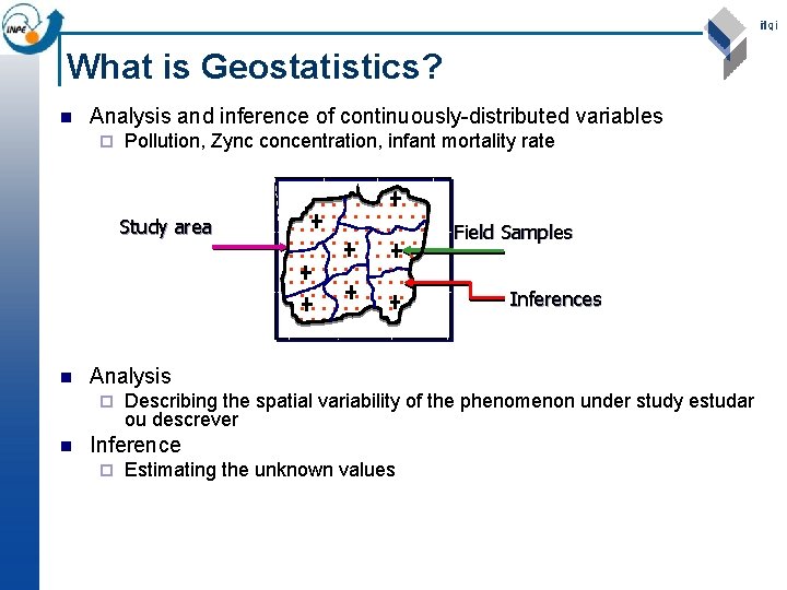
What is Geostatistics? n Analysis and inference of continuously-distributed variables ¨ Pollution, Zync concentration, infant mortality rate Study area n • • • • • • • • • • • • • • • • • • • • • • • Field Samples Inferences Analysis ¨ n • • • • Describing the spatial variability of the phenomenon under study estudar ou descrever Inference ¨ Estimating the unknown values

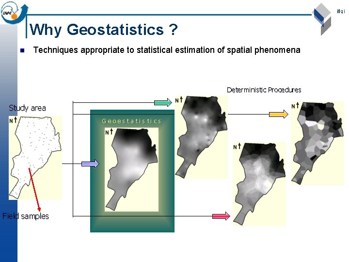
Why Geostatistics ? n Techniques appropriate to statistical estimation of spatial phenomena Deterministic Procedures Study area Geoestatistics Field samples

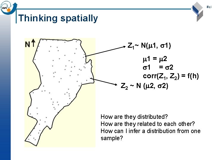
Thinking spatially Z 1~ N( 1, 1) 1 = 2 corr(Z 1, Z 2) = f(h) Z 2 ~ N ( 2, 2) How are they distributed? How are they related to each other? How can I infer a distribution from one sample?

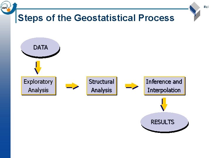
Steps of the Geostatistical Process DATA Exploratory Analysis Structural Analysis Inference and Interpolation RESULTS

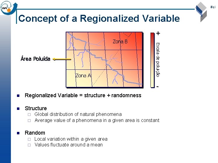
Concept of a Regionalized Variable + Área Poluída Zona A Escala de poluição Zona B n Regionalized Variable = structure + randomness n Structure ¨ ¨ n Global distribution of natural phenomena Average value of a phenomena in a given area is constant Random ¨ ¨ Local variation within a given area Values fluctuate around a mean

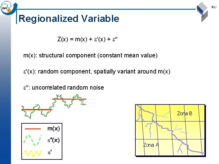
Regionalized Variable Z(x) = m(x) + m(x): structural component (constant mean value) (x): random component, spatially variant around m(x) : uncorrelated random noise Zona B m(x) ”(x) ’ Zona A

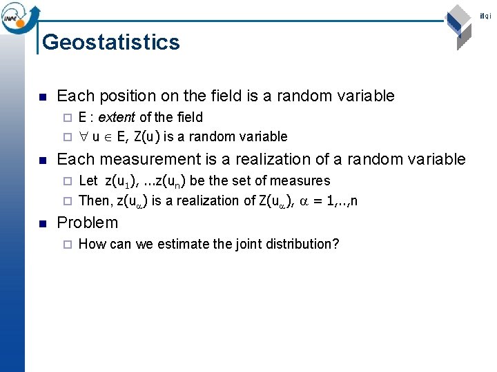
Geostatistics n Each position on the field is a random variable E : extent of the field ¨ u E, Z(u) is a random variable ¨ n Each measurement is a realization of a random variable Let z(u 1), . . . z(un) be the set of measures ¨ Then, z(u ) is a realization of Z(u ), = 1, . . , n ¨ n Problem ¨ How can we estimate the joint distribution?

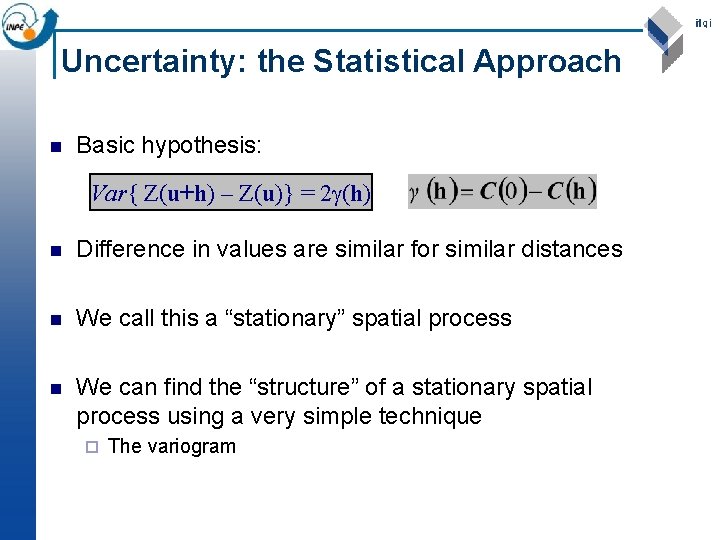
Uncertainty: the Statistical Approach n Basic hypothesis: Var{ Z(u+h) – Z(u)} = 2 (h) n Difference in values are similar for similar distances n We call this a “stationary” spatial process n We can find the “structure” of a stationary spatial process using a very simple technique ¨ The variogram

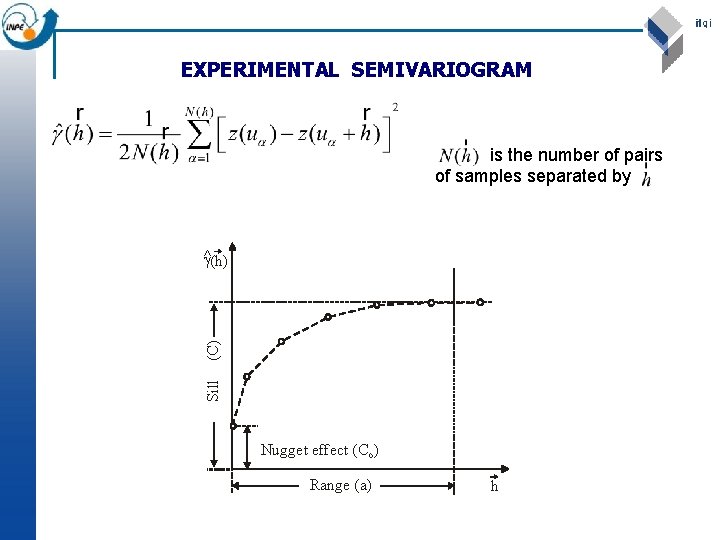
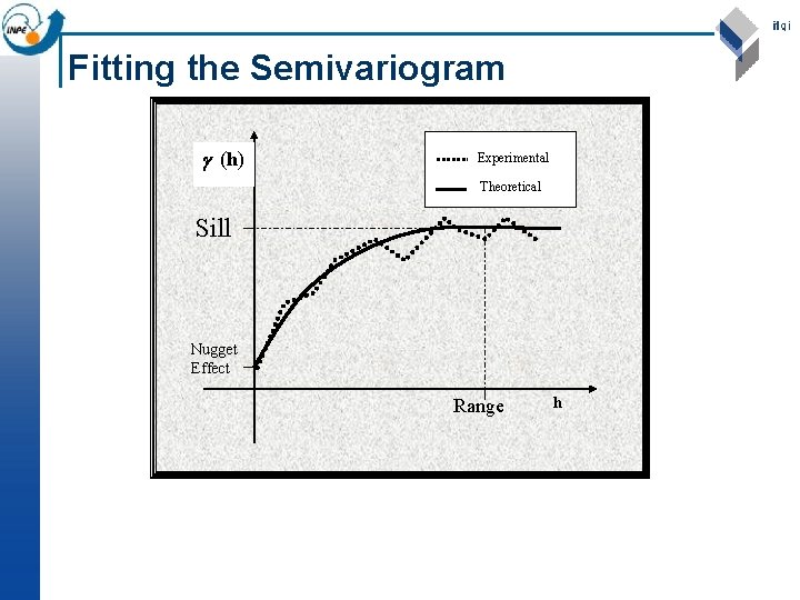
EXPERIMENTAL SEMIVARIOGRAM is the number of pairs of samples separated by Sill (C) ^ (h) Nugget effect (Co) Range (a) h

Building the Experimental Semivariogram n Step 1 (optional): Transforming area maps in samples

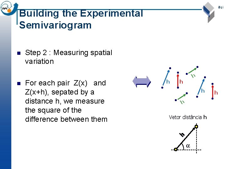
Building the Experimental Semivariogram n Step 2 : Measuring spatial variation For each pair Z(x) and Z(x+h), sepated by a distance h, we measure the square of the difference between them • • h • h • • h • • • h Vetor distância h h n • h

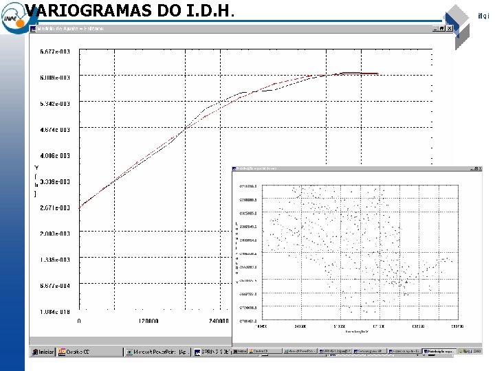
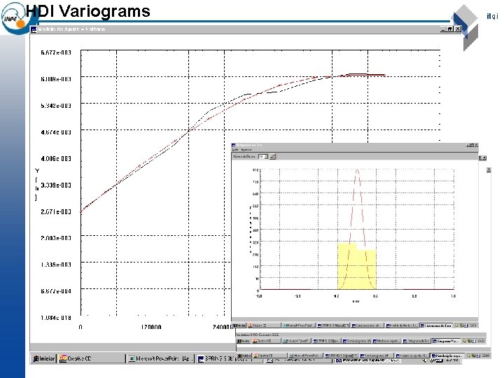
VARIOGRAMAS DO I. D. H.

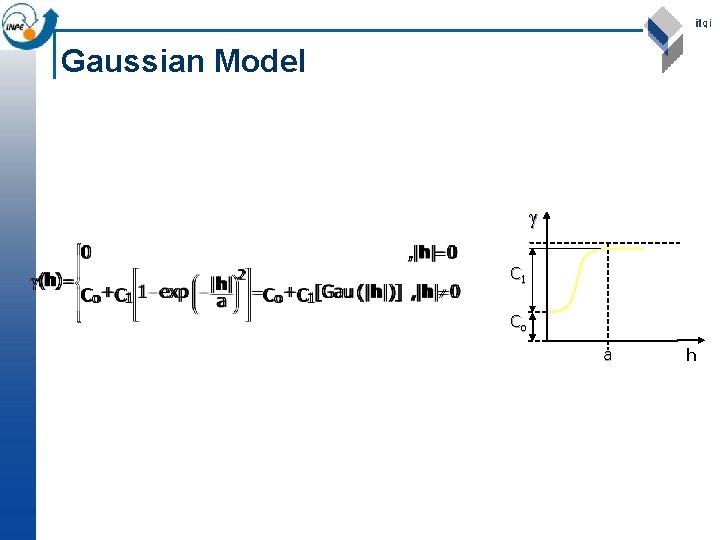
Spatial Model Fitting for Variograms n After building an experimental variogram, we need to fit a theoretical function in order to model the spatial variation n The adjustment procedure is interactive, where the user selects theoretical model that best fits his data. n Some useful models: ¨ Gaussian, Exponential, Spherical models

Fitting the Semivariogram (h) Experimental Theoretical Sill Nugget Effect Range h

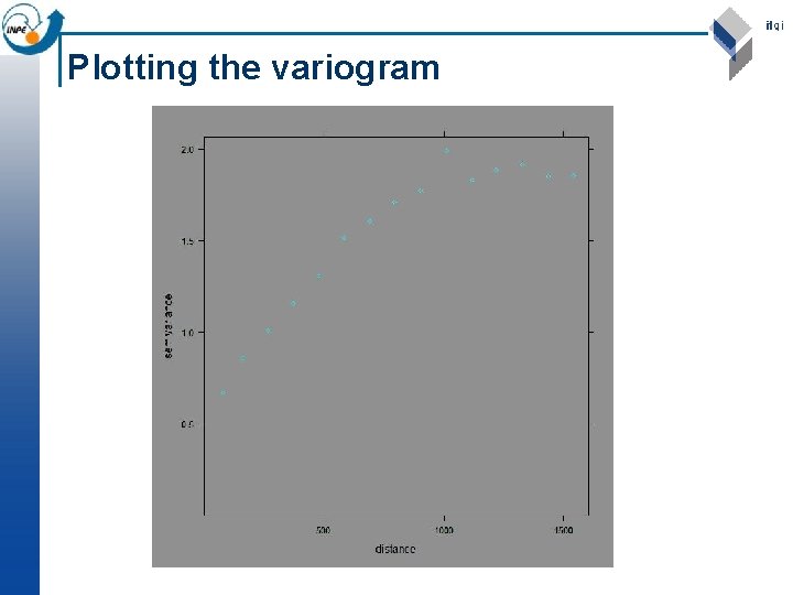
Plotting the variogram

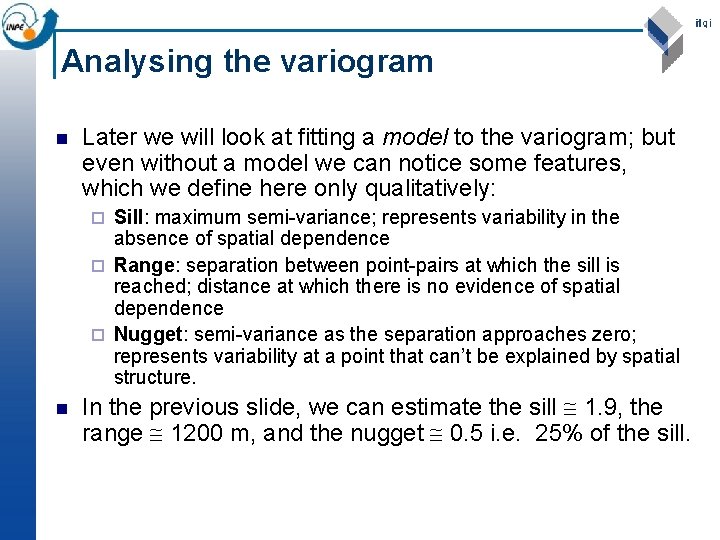
Analysing the variogram n Later we will look at fitting a model to the variogram; but even without a model we can notice some features, which we define here only qualitatively: Sill: maximum semi-variance; represents variability in the absence of spatial dependence ¨ Range: separation between point-pairs at which the sill is reached; distance at which there is no evidence of spatial dependence ¨ Nugget: semi-variance as the separation approaches zero; represents variability at a point that can’t be explained by spatial structure. ¨ n In the previous slide, we can estimate the sill 1. 9, the range 1200 m, and the nugget 0. 5 i. e. 25% of the sill.

Using the experimental variogram to model the random process n Notice that the semivariance of the separation vector (h) is now given as the estimate of covariance in the spatial field. n So it models the spatially-correlated component of the regionalized variable n We must go from the experimental variogram to a variogram model in order to be able to model the random process at any separation.

Modelling the variogram n From the empirical variogram we now derive a variogram model which expresses semivariance as a function of separation vector. It allows us to: n Infer the characteristics of the underlying process from the functional form and its parameters; n Compute the semi-variance between any point-pair, separated by any vector; n Interpolate between sample points using an optimal interpolator (“kriging”)

“Authorized” Models n n Any variogram function must be able to model the following: 1. Monotonically increasing ¨ n n n possibly with a fluctuation (hole) 2. Constant or asymptotic maximum (sill) 3. Non-negative intercept (nugget) 4. Anisotropy Variograms must obey mathematical constraints so that the resulting kriging equations are solvable (e. g. , positive definite between-sample covariance matrices). The permitted functions are called authorized models.

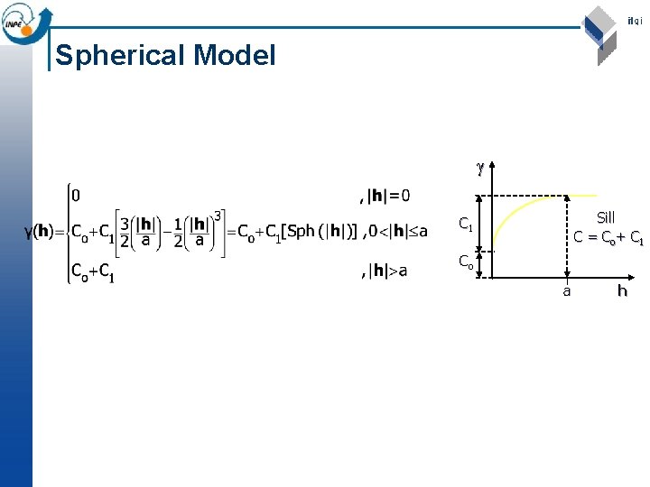
Spherical Model Sill C = C o+ C 1 Co a h

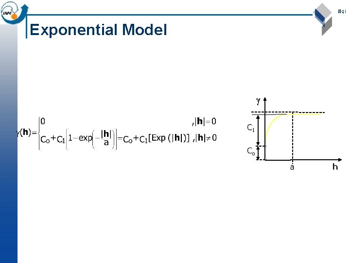
Exponential Model C 1 Co a h

Gaussian Model C 1 Co a h

What sample size to fit a variogram model? n Can’t use non-spatial formulas for sample size, because spatial samples are correlated, and each sample is used multiple times in the variogram estimate ¨ ¨ ¨ No way to estimate the true error, since we have only one realisation Stochastic simulation from an assumed true variogram suggests: < 50 points: not at all reliable 100 to 150 points: more or less acceptable > 250 points: almost certaintly reliable n More points are needed to estimate an anisotropic variogram. n This is very worrying for many environmental datasets (soil cores, vegetation plots, . . . ) especially from short-term fieldwork, where sample sizes of 40 – 60 are typical. Should variograms even be attempted on such small samples?

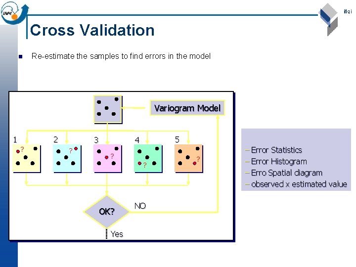
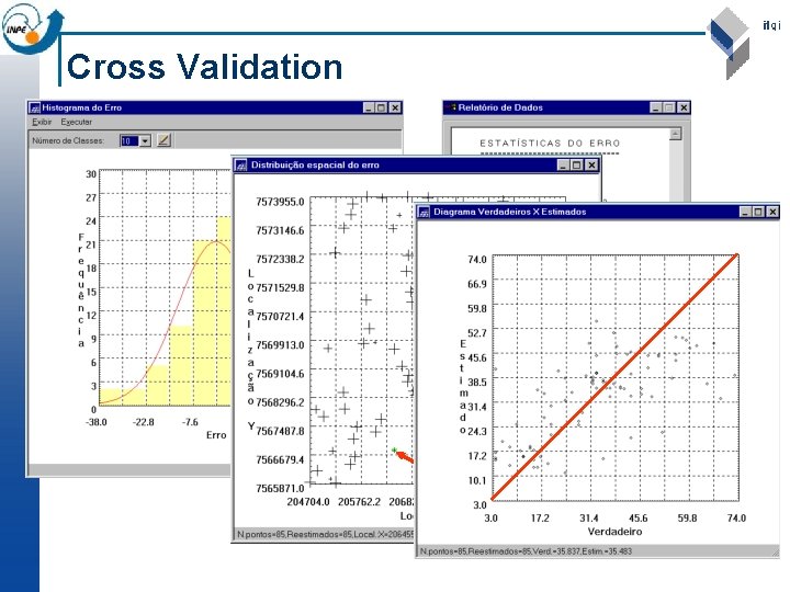
Cross Validation n Re-estimate the samples to find errors in the model Variogram Model 1 2 ? 3 ? 5 4 ? ? OK? Yes NO ? – Error Statistics – Error Histogram – Erro Spatial diagram – observed x estimated value

Cross Validation

Approaches to spatial prediction n n This is the prediction of the value of some variable at an unsampled point, based on the values at the sampled points. This is often called interpolation, but strictly speaking that is only for points that are geographically inside the sample set (otherwise it is extrapolation.

Approaches to prediction: Local predictors n Value of the variable is predicted from “nearby” samples Example: concentrations of soil constituents (e. g. salts, pollutants) ¨ Example: vegetation density ¨

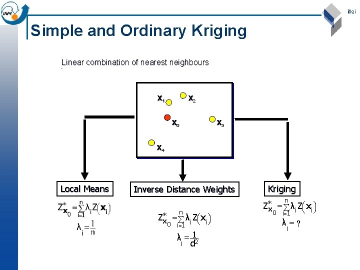
Local Predictors n Each interpolator has its own assumptions, i. e. theory of spatial variability ¨ Nearest neighbour Average within a radius Average of n nearest neighbours Distance-weighted average within a radius Distance-weighted average of n nearest neighbours ¨ Optimal” weighting -> Kriging ¨ ¨

Ordinary Kriging n The theory of regionalised variables leads to an “optimal” interpolation method, in the sense that the prediction variance is minimized. n This is based on theory of random functions, and requires certain assumptions.

Optimal local interpolation: motivation n Problems with average-in-circle methods: ¨ n 1. No objective way to select radius of circle or number of points Problems with inverse-distance methods: 1. How to choose power (inverse, inverse squared. . . )? ¨ 2. How to choose limiting radius? ¨ n In both cases: 1. Uneven distribution of samples could over– or under– emphasize some parts of the field ¨ 2. prediction error must be estimated from a separate validation dataset ¨

An “optimal” local predictor would have these features: n n n n Prediction is made as a linear combination of known data values (a weighted average). Prediction is unbiased and exact at known points Points closer to the point to be predicted have larger weights Clusters of points “reduce to” single equivalent points, i. e. , over-sampling in a small area can’t bias result Closer sample points “mask” further ones in the same direction Error estimate is based only on the sample configuration, not the data values Prediction error should be as small as possible.

Kriging n n A “Best Linear Unbiased Predictor” (BLUP) that satisfies certain criteria for optimality. It is only “optimal” with respect to the chosen model! Based on theory of random processes, with covariances depending only on separation (i. e. a variogram model) Theory developed several times (Kolmogorov 1930’s, Wiener 1949) but current practise dates back to Matheron (1963), formalizing the practical work of the mining engineer D G Krige (RSA).

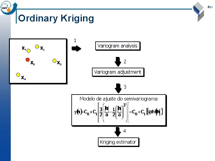
How do we use Kriging? n n 1. Sample, preferably at different resolutions 2. Calculate the experimental variogram 3. Model the variogram with one or more authorized functions 4. Apply the kriging system, with the variogram model of spatial dependence, at each point to be predicted Predictions are often at each point on a regular grid (e. g. a raster map) ¨ These ‘points’ are actually blocks the size of the sampling support ¨ Can also predict in blocks larger than the original support ¨ n 5. Calculate the error of each prediction; this is based only on the sample point locations, not their data values.

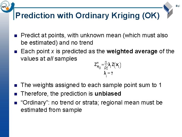
Prediction with Ordinary Kriging (OK) n In OK, we model the value of variable z at location si as the sum of a regional mean m and a spatiallycorrelated random component e(si): n Z(si) = m+e(si) n The regional mean m is estimated from the sample, but not as the simple average, because there is spatial dependence. It is implicit in the OK system.

Prediction with Ordinary Kriging (OK) n n Predict at points, with unknown mean (which must also be estimated) and no trend Each point x is predicted as the weighted average of the values at all samples n Z*x = å λi Zæçè xi ö÷ø 0 i=1 λ =? i n n n The weights assigned to each sample point sum to 1 Therefore, the prediction is unbiased “Ordinary”: no trend or strata; regional mean must be estimated from sample

Simple and Ordinary Kriging Linear combination of nearest neighbours • x 1 x 2 x 0 x 3 x 4 Local Means Inverse Distance Weights Kriging n n Z*x = å λi Zæçè xi ö÷ø i=1 λ =? Z*x = å λi Zæçè xi ö÷ø 0 λ = 12 i d 0 i=1 i

Ordinary Kriging 1 x 2 x 0 x 4 x 3 Variogram analysis 2 Variogram adjustment 3 Modelo de ajuste do semivariograma 4 Kriging estimator

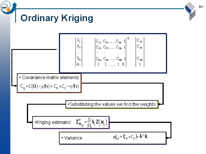
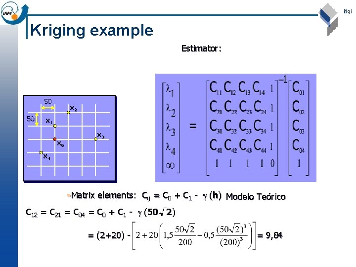
Ordinary Kriging l 1 l 2 : ln = C 11 C 21 : C n 1 1 C 12. . C 1 n 1 C 22. . C 2 n 1 : : : C n 2. . C nn 1 1. . 1 0 -1 C 10 C 20 : C n 0 1 • Covariance matrix elements Cij = C(0) - γ (h) = C 0 + C 1 - γ (h) • Substituting the values we find the weights n • Kriging estimator: Z*x = å λi Zæçè xi ö÷ø 0 i=1 • Variance 2 = (C 0 + C 1 )- λ T k σko

Kriging example Estimator: 50 50 x 2 x 1 x 0 x 3 x 4 • Matrix elements: Cij = C 0 + C 1 - (h) Modelo Teórico C 12 = C 21 = C 04 = C 0 + C 1 - (50 2) = (2+20) - = 9, 84

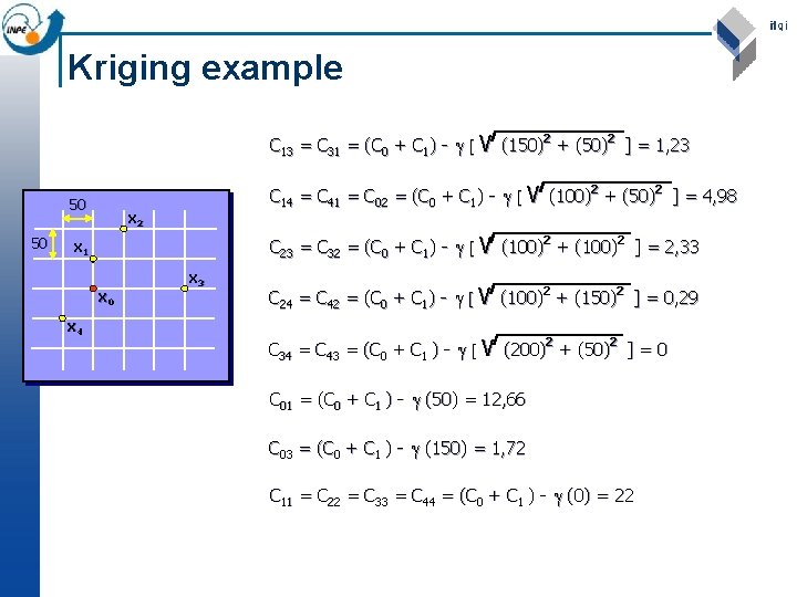
Kriging example C 13 = C 31 = (C 0 + C 1) - [ V (150) 2 + (50) 2 ] = 1, 23 2 C 14 = C 41 = C 02 = (C 0 + C 1) - [ V (100) 2 + (50) 2 ] = 4, 98 2 50 50 x 2 2 C 23 = C 32 = (C 0 + C 1) - [ V (100) 2 + (100) 2 ] = 2, 33 2 x 1 x 0 x 4 2 x 3 2 C 24 = C 42 = (C 0 + C 1) - [ V (100) 2 + (150) 2 ] = 0, 29 2 2 C 34 = C 43 = (C 0 + C 1 ) - [ V (200) 2 + (50) 2 ] = 0 2 2 C 01 = (C 0 + C 1 ) - (50) = 12, 66 C 03 = (C 0 + C 1 ) - (150) = 1, 72 C 11 = C 22 = C 33 = C 44 = (C 0 + C 1 ) - (0) = 22

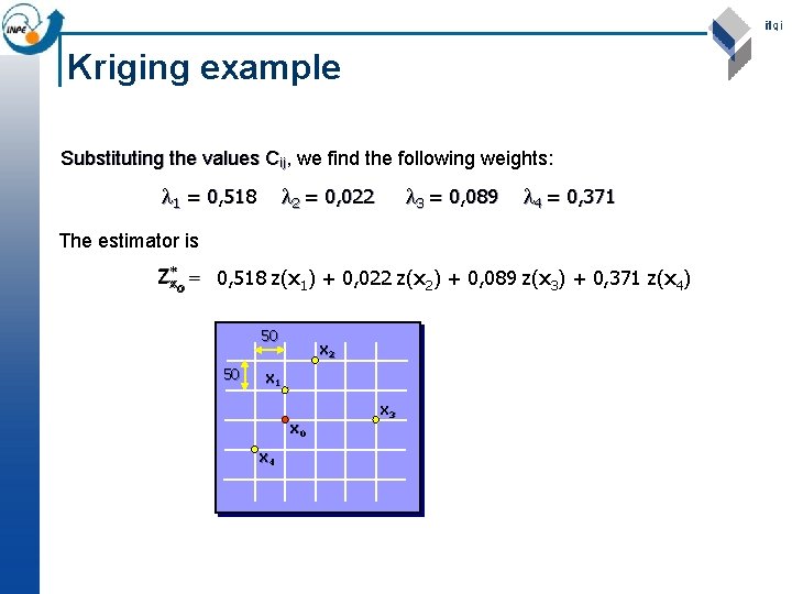
Kriging example Substituting the values Cij, we find the following weights: l 1 = 0, 518 l 2 = 0, 022 l 3 = 0, 089 l 4 = 0, 371 The estimator is Z*x o = 0, 518 z(x 1) + 0, 022 z(x 2) + 0, 089 z(x 3) + 0, 371 z(x 4) 50 50 x 2 x 1 x 0 x 4 x 3

Sampling configurations n n n There is no agreement on a “universally” optimal sampling configuration for geostatistical research (i. e. , variogram modelling, followed by spatial prediction), but: for spatial prediction, regular (lattice, or triangular) sampling is optimal (in case of isotropy; otherwise stretched lattices); for variogram modelling, all distances should be present, including sufficient information about short distances (which are not present when sampling regularly) cross validation on a regular sampling grid will not reveal deficiencies in modelled short distance behaviour of the variogram; interpolated maps will be dominated by this short distance variogram behaviour. compromise: most effort put to regular spread, sufficient effort to short distance replicates. related questions: adding sampling points to an existing design, or reducing (“optimizing”) an existing monitoring network.

Questions about kriging n n n what do sill, nugget, range, and anisotropy tell about spatial variability of an observed variable? what happens if we predict a value at an observation location? what does the prediction variance measure? why is the interpolator discontinuous at observation locations when the nugget is positive? why is the prediction variance pattern independent on data, but only dependent on data configuration? what are the causes for positive nugget effect?

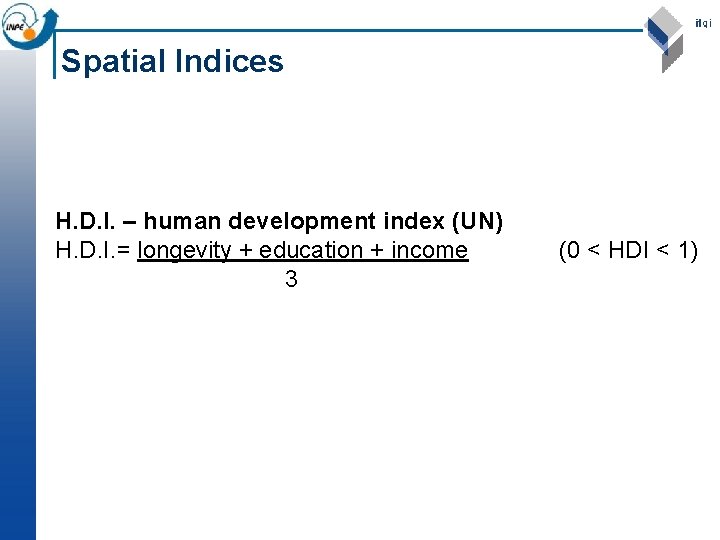
Spatial Indices H. D. I. – human development index (UN) H. D. I. = longevity + education + income 3 (0 < HDI < 1)

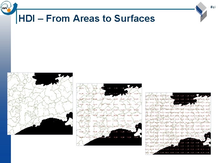
HDI – From Areas to Surfaces

HDI Variograms

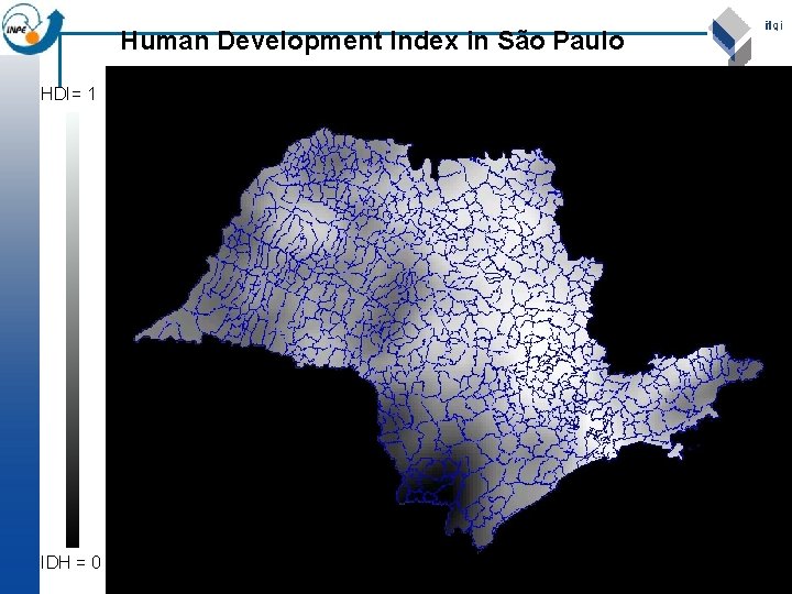
Human Development Index in São Paulo HDI= 1 IDH = 0

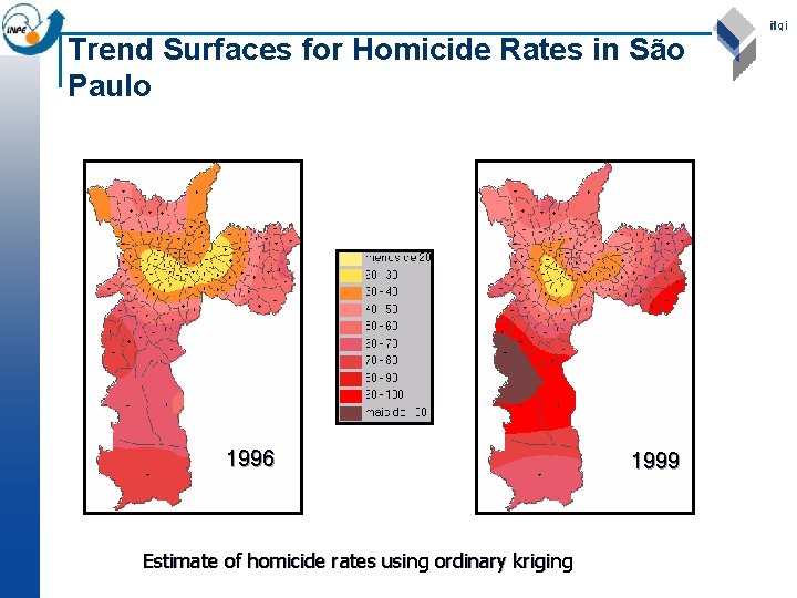
Trend Surfaces for Homicide Rates in São Paulo 1996 Estimate of homicide rates using ordinary kriging 1999

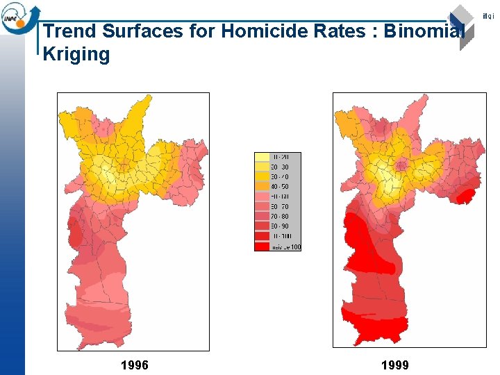
Trend Surfaces for Homicide Rates : Binomial Kriging 1996 1999

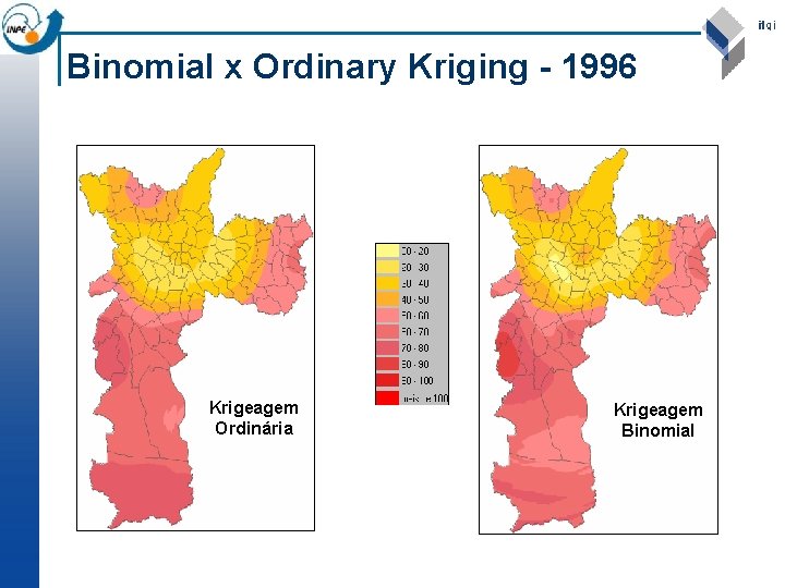
Binomial x Ordinary Kriging - 1996 Krigeagem Ordinária Krigeagem Binomial

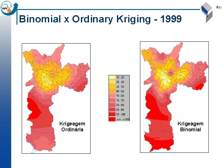
Binomial x Ordinary Kriging - 1999 Krigeagem Ordinária Krigeagem Binomial

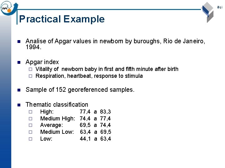
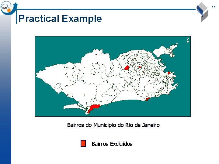
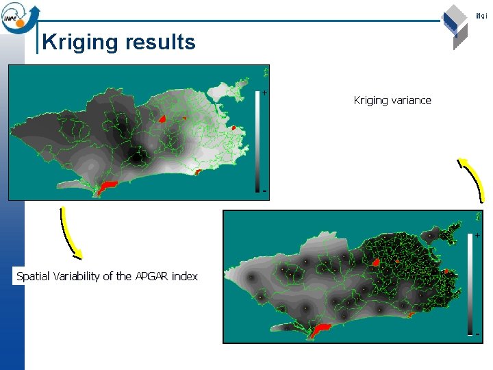
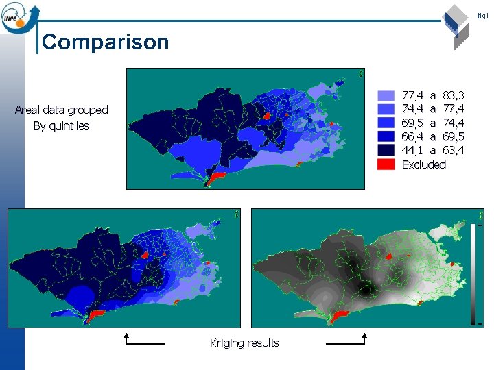
Practical Example n Analise of Apgar values in newborn by buroughs, Rio de Janeiro, 1994. n Apgar index ¨ ¨ Vitality of newborn baby in first and fifth minute after birth Respiration, heartbeat, response to stimula n Sample of 152 georeferenced samples. n Thematic classification ¨ ¨ ¨ High: Medium High: Average: Medium Low: 77, 4 74, 4 69, 5 63, 4 44, 1 a a a 83, 3 77, 4 74, 4 69, 5 63, 4

Practical Example Bairros do Municipio do Rio de Janeiro Bairros Excluídos

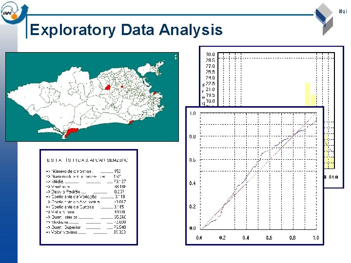
Exploratory Data Analysis

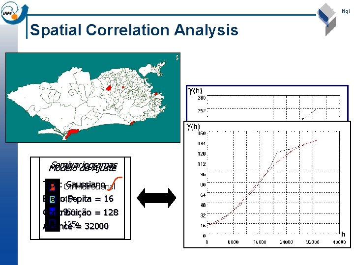
Spatial Correlation Analysis Semivariogramas Modelo de Ajuste Tipo: Omnidirecional Gaussiano o Efeito 45 Pepita = 16 90 o Contribuição = 128 o 135= Alcance 32000

Kriging results + Kriging variance - + Spatial Variability of the APGAR index -

Comparison 77, 4 a 83, 3 74, 4 a 77, 4 69, 5 a 74, 4 66, 4 a 69, 5 44, 1 a 63, 4 Excluded Areal data grouped By quintiles + Kriging results