Spatial Analysis Grid cell counts Grid Methods Data

Spatial Analysis Grid cell counts

Grid Methods • Data are recorded as coming from a particular area, but we do not have exact coordinates • Screened artifacts from an excavation unit, census data (population counts from survey tracts, incidence of disease or other characteristic

Spatial Clusters • Null hypothesis is that the data are distributed according to a Poisson distribution • Variance/mean ratio (VMR) provides a rough indication of clustering where VMR = 1 is a Poisson distribution, <1 is regular and >1 clustered

Visualizing Counts • Choropleth maps represent quantity or category by shading polygons • Dot density maps represent quantity/density by randomly or regularly spaced symbols within the polygon

Package sp • Definitions for spatial objects • Spatial. Polygons are an object that contains a set of places (e. g. grid cells, states, counties) each of which can include multiple polygons and/or holes • Perfect for choropleth and dot density maps

# Create a Spatial Polygons object source("Grid. Units 3 a. R") # Append first line of coordinates to the bottom so # first-coord = last-coord Quads <- lapply(Quads, function(x) rbind(x, x[1, ])) # Load package sp for spatial classes library(sp) # Create Polygon list (one from each unit) Quads. List <- lapply(Quads, function(x) Polygon(x, hole=FALSE)) # Areas 3 a <- sapply(Quads. List, function(x) x@area) to get areas # Create a Polygons list Units <- lapply(1: 20, function(x) Polygons(Quads. List[x], Unit. Lbl[x])) # Create a Spatial Polygons list SPUnits <- Spatial. Polygons(Units, 1: 20) # sapply(1: 20, function(x) SPUnits@polygons[[x]]@area) # to get areas from Spatial. Polygons

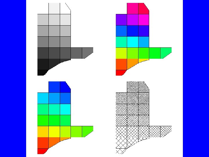
opar <- par(mfrow=c(2, 2), mar=c(0, 0, 0, 0)) plot(SPUnits, col=gray(1: 20/20)) plot(SPUnits, col=rainbow(20, start=0, end=4/6)) plot(SPUnits, density=c(6: 25), angle=c(45, -45)) plot(SPUnits, density=c(6: 25), angle=c(-45, 45), add=TRUE) par(opar)

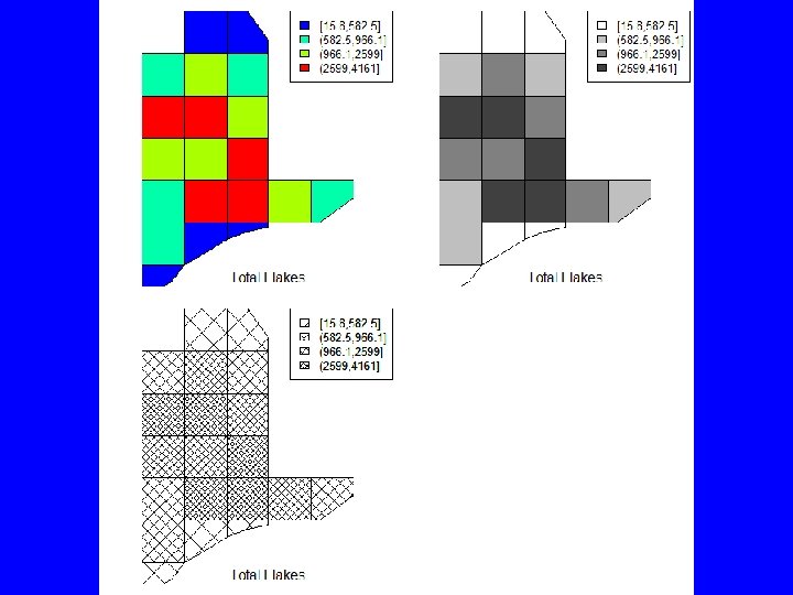
# Load Flk. Size 3 a Flk. Den 3 a <- round(sweep(Flk. Size 3 a[, c("TCt", "TWgt")], 1, Flk. Size 3 a$Area, "/"), 1) Flk. Den 3 a <- data. frame(East=Flk. Size 3 a$East, North=Flk. Size 3 a$North, Flk. Den 3 a) var(Flk. Den 3 a$TCt)/mean(Flk. Den 3 a$TCt) # Cut into 4 groups TCt. Grp 1 <- cut(Flk. Den 3 a$TCt, quantile(Flk. Den 3 a$TCt, c(0: 4/4)), include. lowest=TRUE, dig=4) # TCt. Grp 2 <- cut(Flk. Den 3 a$TCt, quantile(Flk. Den 3 a$TCt, c(0: 4/4)), # labels=1: 4, include. lowest=TRUE) # TCt. Grp 3 <- cut(Flk. Den 3 a$TCt, 0: 4*1250+25, include. lowest=TRUE, # dig=4) Colors <- rev(rainbow(4, start=0, end=4/6)) Gray <- rev(gray(1: 4/4)) Hatch <- c(5, 10, 15, 20)

opar <- par(mfrow=c(2, 2), mar=c(0, 0, 0, 0)) plot(SPUnits, col=Colors[as. numeric(TCt. Grp 1)]) text(985, 1015. 75, "Total Flakes", cex=1. 25) legend(985. 5, 1022, levels(TCt. Grp 1), fill=Colors) plot(SPUnits, col=Gray[as. numeric(TCt. Grp 1)]) text(985, 1015. 75, "Total Flakes", cex=1. 25) legend(985. 5, 1022, levels(TCt. Grp 1), fill=Gray) plot(SPUnits, angle=45, density=Hatch[as. numeric(TCt. Grp 1)]) plot(SPUnits, angle=-45, density=Hatch[as. numeric(TCt. Grp 1)], add=TRUE) text(985, 1015. 75, "Total Flakes", cex=1. 25) legend(985. 5, 1022, levels(TCt. Grp 1), angle=45, density=Hatch) legend(985. 5, 1022, levels(TCt. Grp 1), angle=-45, density=Hatch) par(opar)

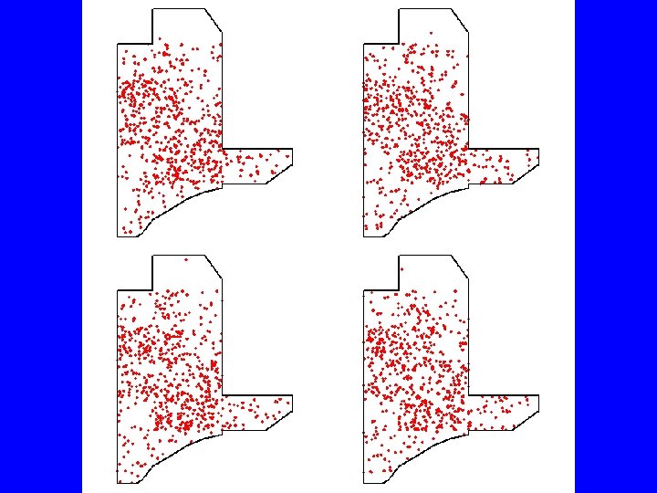
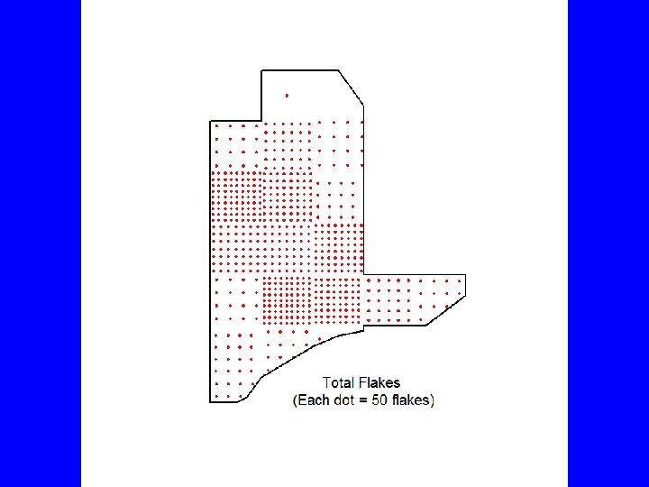
library(maptools) opar <- par(mfrow=c(2, 2), mar=c(0, 0, 0, 0)) for (i in 1: 4) { dots <- dots. In. Polys(SPUnits, as. integer(round(Flk. Den 3 a$TCt/50, 0))) # 1 dot = 50 flakes plot(SPUnits, lty=0) points(dots, pch=20, col="red") polygon(c(982, 983, 984. 5, 985, 987, 986. 2, 985, 984, 983. 5, 983, 982. 7, 982. 5), c(1015. 5, 1021, 1022, 1021. 3, 1018, 1017. 6, 1017, 1016. 9, 1016. 8, 1016. 6, 1016. 3, 1016, 1015. 5), lwd=2, border="black") } par(opar) dots <- dots. In. Polys(SPUnits, as. integer(round(Flk. Den 3 a$TCt/50, 0)), f="regular") plot(SPUnits, lty=0) points(dots, pch=20, cex=. 75, col="red") polygon(c(982, 983, 984. 5, 985, 987, 986. 2, 985, 984, 983. 5, 983, 982. 7, 982. 5), c(1015. 5, 1021, 1022, 1021. 3, 1018, 1017. 6, 1017, 1016. 9, 1016. 8, 1016. 6, 1016. 3, 1016, 1015. 5), lwd=2, border="black") text(985, 1015. 75, "Total Flakes n(Each dot = 50 flakes)", cex=1. 25)

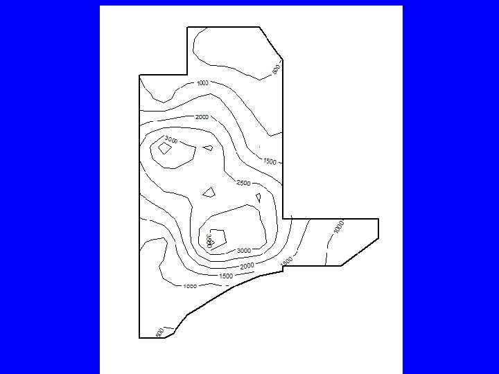
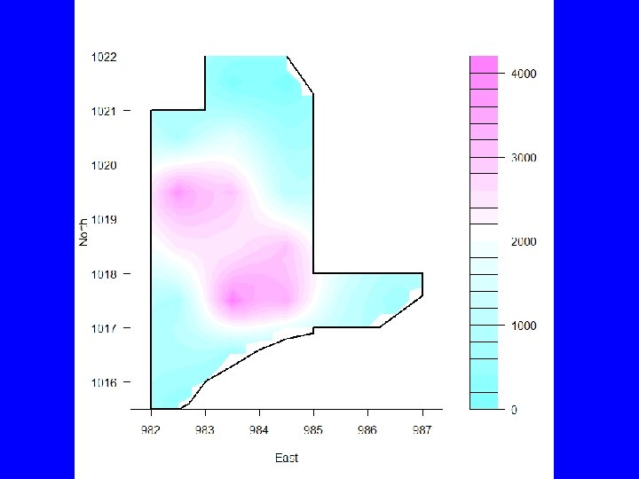
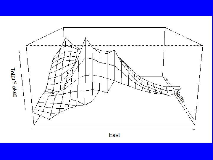
Countour Mapping • We fit a model to the data to interpolate between the observations and smooth them – Trend surface models with polynomials – Kriging – developed in geophysics to interpolate and extrapolate

library(geo. R) # load Flk. Den 3 a. RData Flk. Den 3 a$East <- Flk. Den 3 a$East +. 5 Flk. Den 3 a$North <- Flk. Den 3 a$North +. 5 Flk. Den 3 a$Av. Wgt <- Flk. Den 3 a$TWgt/Flk. Den 3 a$TCt columns <- names(Flk. Den 3 a) Flakes 3 a <- as. geodata(Flk. Den 3 a, 1: 2, 3: 5, c("TCt", "TWgt", "Av. Wgt")) Grid. Pts <- expand. grid(East=seq(982, 987, . 25), North=seq(1015. 5, 1022, . 25)) Border 3 a <- cbind(c(982, 983, 984. 5, 985, 987, 986. 2, 985, 984, 983. 5, 983, 982. 7, 982. 5), c(1015. 5, 1021, 1022, 1021. 3, 1018, 1017. 6, 1017, 1016. 9, 1016. 8, 1016. 6, 1016. 3, 1016, 1015. 5)) V <- variog(Flakes 3 a, data=Flakes 3 a$data[, "TCt"]) plot(V, type="b") vf <- variofit(V) TCt. Kv <- krige. conv(Flakes 3 a, data=Flakes 3 a$data[, "TCt"], locations=Grid. Pts, krige=krige. control(cov. pars=c(1292000, . 824))) contour(TCt. Kv, borders=Border 3 a, xlab="East", ylab="North") contour(TCt. Kv, borders=Border 3 a, axes=FALSE) contour(TCt. Kv, borders=Border 3 a, filled=TRUE) persp(TCt. Kv, borders=Border 3 a, xlab="East", ylab="North", zlab="Total Flakes", expand=. 5)

Unconstrained Clustering • Proposed by Robert Whallon • Take grid data and computer percentages (areas defined by relative abundance, not density) • Cluster grids and plot the distribution of the clusters to identify activity areas