Spatial Analysis 1 Digital Elevation Model DEM 2

Spatial Analysis 1

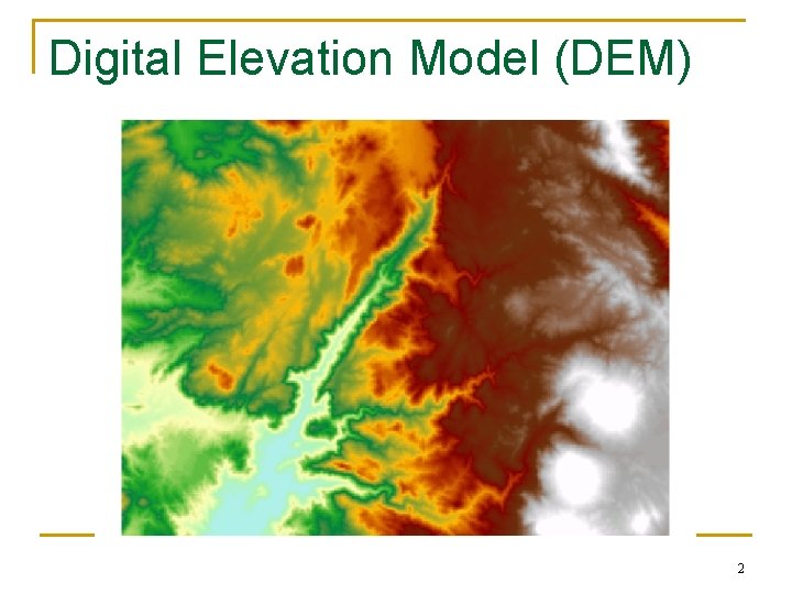
Digital Elevation Model (DEM) 2

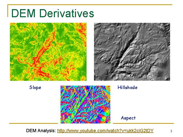
DEM Derivatives Slope Hillshade Aspect DEM Analysis: http: //www. youtube. com/watch? v=ukk 2 ci. G 2 t. DY 3

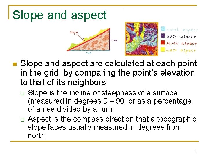
Slope and aspect n Slope and aspect are calculated at each point in the grid, by comparing the point’s elevation to that of its neighbors q q Slope is the incline or steepness of a surface (measured in degrees 0 – 90, or as a percentage of a rise divided by a run) Aspect is the compass direction that a topographic slope faces usually measured in degrees from north 4

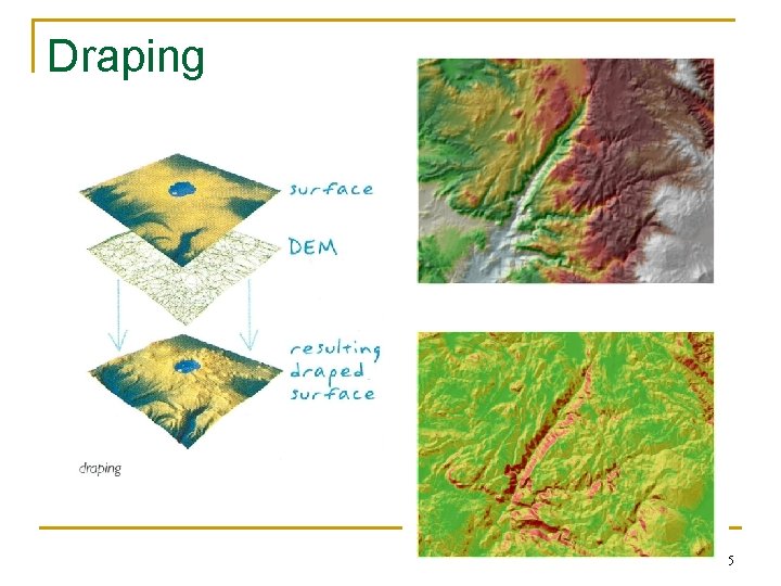
Draping 5

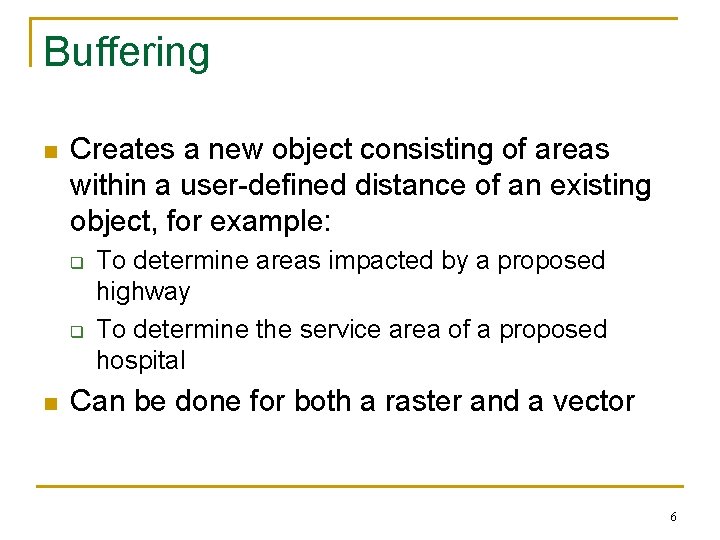
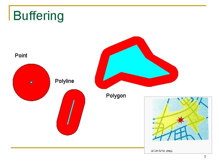
Buffering n Creates a new object consisting of areas within a user-defined distance of an existing object, for example: q q n To determine areas impacted by a proposed highway To determine the service area of a proposed hospital Can be done for both a raster and a vector 6

Buffering Point Polyline Polygon 7

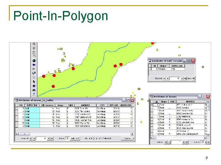
Point-in-polygon transformation n Determine whether a point lies inside or outside a polygon q q generalization: assign many points to containing polygons used to assign crimes to police precincts, voters to voting districts, accidents to reporting counties 8

Point-In-Polygon 9

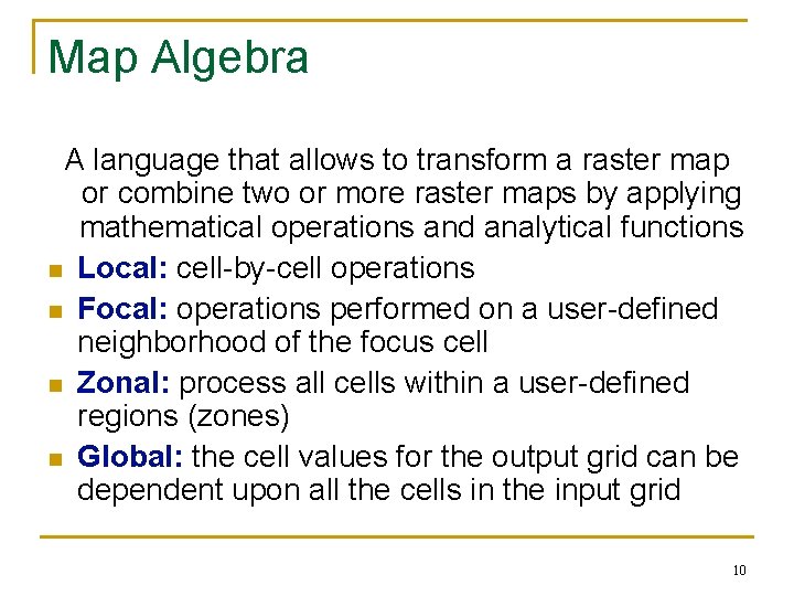
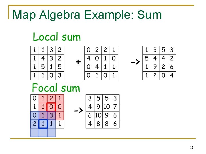
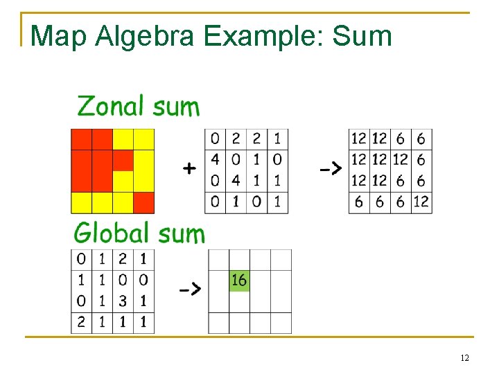
Map Algebra A language that allows to transform a raster map or combine two or more raster maps by applying mathematical operations and analytical functions n Local: cell-by-cell operations n Focal: operations performed on a user-defined neighborhood of the focus cell n Zonal: process all cells within a user-defined regions (zones) n Global: the cell values for the output grid can be dependent upon all the cells in the input grid 10

Map Algebra Example: Sum 11

Map Algebra Example: Sum 12

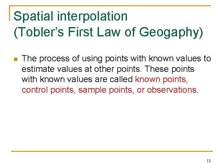
Spatial interpolation (Tobler’s First Law of Geogaphy) n The process of using points with known values to estimate values at other points. These points with known values are called known points, control points, sample points, or observations. 13

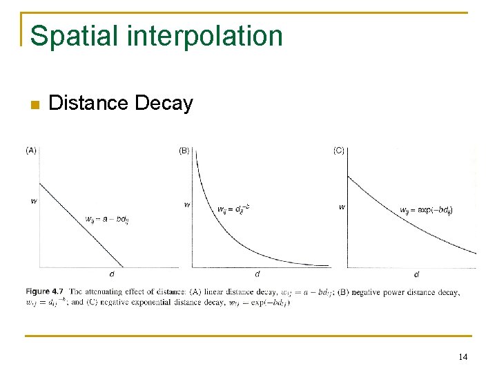
Spatial interpolation n Distance Decay 14

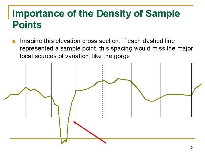
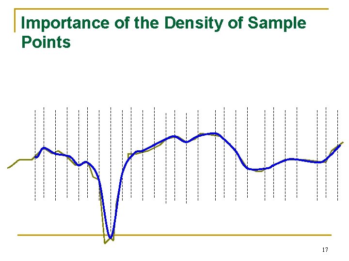
Importance of the Density of Sample Points n Imagine this elevation cross section: If each dashed line represented a sample point, this spacing would miss the major local sources of variation, like the gorge 15

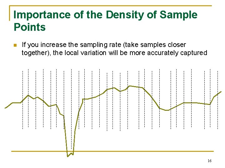
Importance of the Density of Sample Points n If you increase the sampling rate (take samples closer together), the local variation will be more accurately captured 16

Importance of the Density of Sample Points 17

Kriging n n Kriging is a spatial interpolation technique that assumes that the spatial variation of an attribute may consist of three components: a spatially correlated component, representing the variation of the regionalized variable; a ‘drift’ or structure, representing a trend; and a random error term. Developed by Georges Matheron to evaluate new GOLD mines with a limited number of borholes. 18

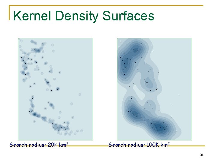
Density estimation n n Spatial interpolation is used to fill the gaps in a field Density estimation creates a field from discrete objects. The field’s value at any point is an estimate of the density of discrete objects at that point q E. g. estimating a map of population density (a field) from a map of individual people (discrete objects) 19

Kernel Density Surfaces Search radius: 20 K km 2 Search radius: 100 K km 2 20