Sparse Signal Processing Trn Duy Trc ECE Department

Sparse Signal Processing Trần Duy Trác ECE Department The Johns Hopkins University Baltimore, MD 21218

Course Overview u Sparse signal processing § Fundamentals: information theory, variable-length coding, quantization, transforms, signal decomposition § Traditional Analysis Viewpoint: transform coding framework; compression; international coding standards § Recent Synthesis viewpoint: linear regression data model, compressed sensing, sparse signal recovery & applications u Goals § Focus on big pictures, key concepts, elegant ideas, not much rigorous mathematical treatment § Provide hands-on experience with simple Matlab exercises § Hopefully lead to future research and developments Fun Fun Fun!

Outline u Signal properties & formats § § § u Analog versus digital Natural signals: properties & formats, color spaces Where does sparsity comes from? General signal coding framework Error & similarity measurements Statistical modeling of natural signals Lossless variable-length coding § Information theory, entropy coding § Huffman coding § Arithmetic coding u Lossy coding via Quantization § Optimal conditions, scalar & embedded quantization

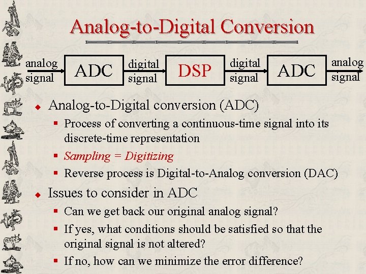
Analog-to-Digital Conversion analog signal u ADC digital signal DSP digital signal ADC analog signal Analog-to-Digital conversion (ADC) § Process of converting a continuous-time signal into its discrete-time representation § Sampling = Digitizing § Reverse process is Digital-to-Analog conversion (DAC) u Issues to consider in ADC § Can we get back our original analog signal? § If yes, what conditions should be satisfied so that the original signal is not altered? § If no, how can we minimize the error difference?

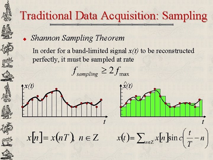
Traditional Data Acquisition: Sampling u Shannon Sampling Theorem In order for a band-limited signal x(t) to be reconstructed perfectly, it must be sampled at rate ^ x(t) t t

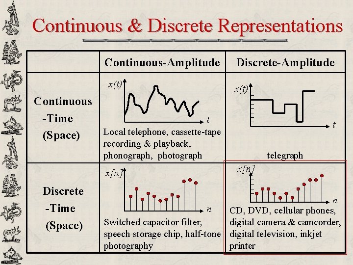
Continuous & Discrete Representations Continuous-Amplitude x(t) Discrete-Amplitude x(t) Continuous -Time t Local telephone, cassette-tape (Space) t recording & playback, phonograph, photograph x[n] Discrete -Time (Space) telegraph x[n] n n CD, DVD, cellular phones, Switched capacitor filter, digital camera & camcorder, speech storage chip, half-tone digital television, inkjet photography printer

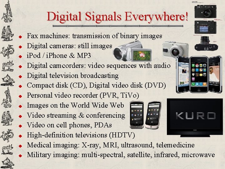
Digital Signals Everywhere! u u u u Fax machines: transmission of binary images Digital cameras: still images i. Pod / i. Phone & MP 3 Digital camcorders: video sequences with audio Digital television broadcasting Compact disk (CD), Digital video disk (DVD) Personal video recorder (PVR, Ti. Vo) Images on the World Wide Web Video streaming & conferencing Video on cell phones, PDAs High-definition televisions (HDTV) Medical imaging: X-ray, MRI, ultrasound, telemedicine Military imaging: multi-spectral, satellite, infrared, microwave

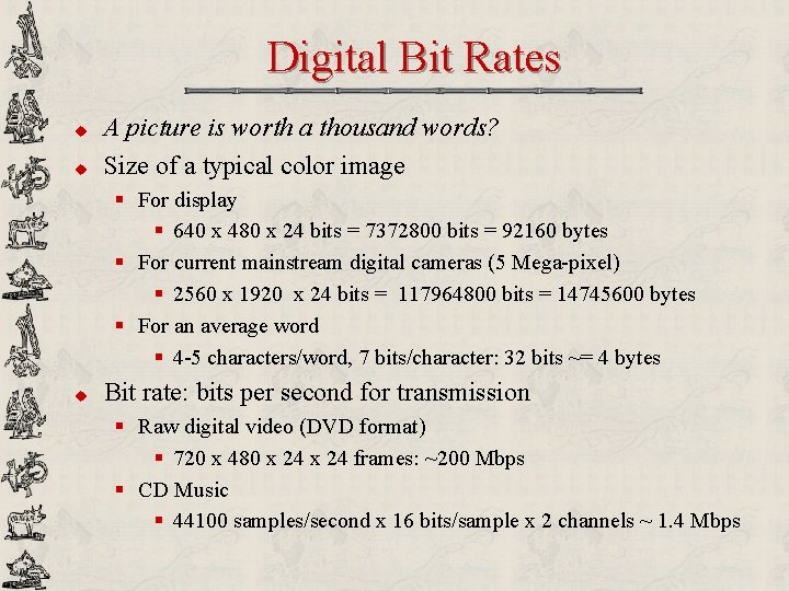
Digital Bit Rates u u A picture is worth a thousand words? Size of a typical color image § For display § 640 x 480 x 24 bits = 7372800 bits = 92160 bytes § For current mainstream digital cameras (5 Mega-pixel) § 2560 x 1920 x 24 bits = 117964800 bits = 14745600 bytes § For an average word § 4 -5 characters/word, 7 bits/character: 32 bits ~= 4 bytes u Bit rate: bits per second for transmission § Raw digital video (DVD format) § 720 x 480 x 24 frames: ~200 Mbps § CD Music § 44100 samples/second x 16 bits/sample x 2 channels ~ 1. 4 Mbps

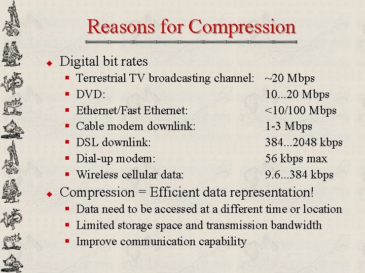
Reasons for Compression u Digital bit rates § § § § u Terrestrial TV broadcasting channel: DVD: Ethernet/Fast Ethernet: Cable modem downlink: DSL downlink: Dial-up modem: Wireless cellular data: ~20 Mbps 10. . . 20 Mbps <10/100 Mbps 1 -3 Mbps 384. . . 2048 kbps 56 kbps max 9. 6. . . 384 kbps Compression = Efficient data representation! § Data need to be accessed at a different time or location § Limited storage space and transmission bandwidth § Improve communication capability

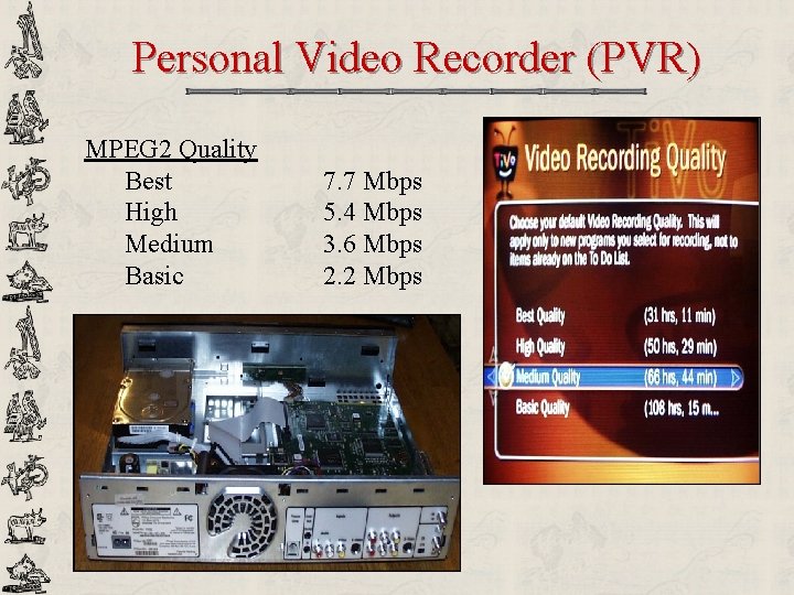
Personal Video Recorder (PVR) MPEG 2 Quality Best High Medium Basic 7. 7 Mbps 5. 4 Mbps 3. 6 Mbps 2. 2 Mbps

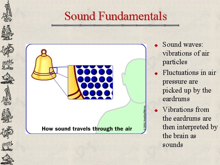
Sound Fundamentals u u u Sound waves: vibrations of air particles Fluctuations in air pressure are picked up by the eardrums Vibrations from the eardrums are then interpreted by the brain as sounds

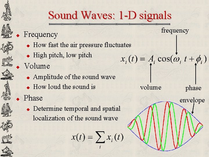
Sound Waves: 1 -D signals u u How fast the air pressure fluctuates High pitch, low pitch Volume u u u frequency Frequency Amplitude of the sound wave How loud the sound is Phase u Determine temporal and spatial localization of the sound wave volume phase envelope

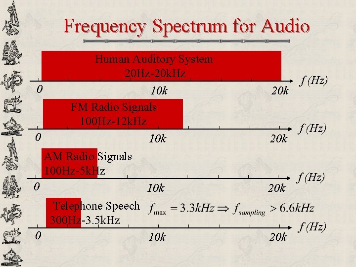
Frequency Spectrum for Audio 0 0 Human Auditory System 20 Hz-20 k. Hz 10 k FM Radio Signals 100 Hz-12 k. Hz 10 k 20 k AM Radio Signals 100 Hz-5 k. Hz 0 10 k 20 k Telephone Speech 300 Hz-3. 5 k. Hz 0 10 k 20 k f (Hz)

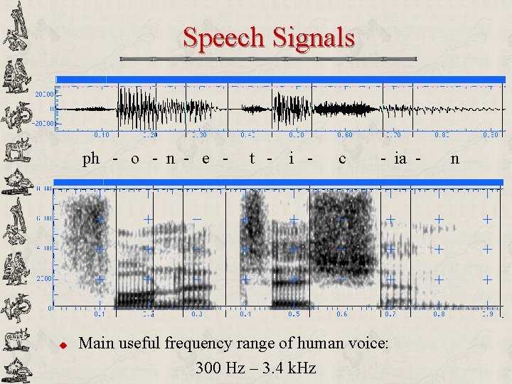
Speech Signals ph - o - n - e - u t - i - c - ia - Main useful frequency range of human voice: 300 Hz – 3. 4 k. Hz n

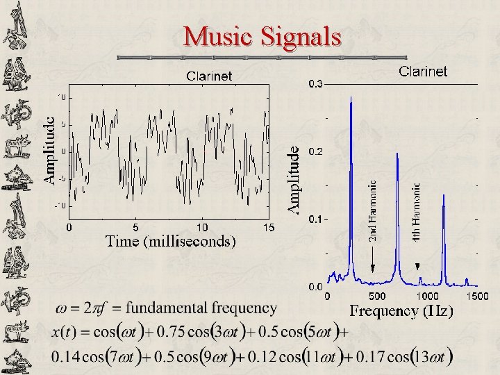
Music Signals

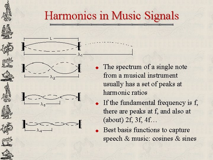
Harmonics in Music Signals u u u The spectrum of a single note from a musical instrument usually has a set of peaks at harmonic ratios If the fundamental frequency is f, there are peaks at f, and also at (about) 2 f, 3 f, 4 f… Best basis functions to capture speech & music: cosines & sines

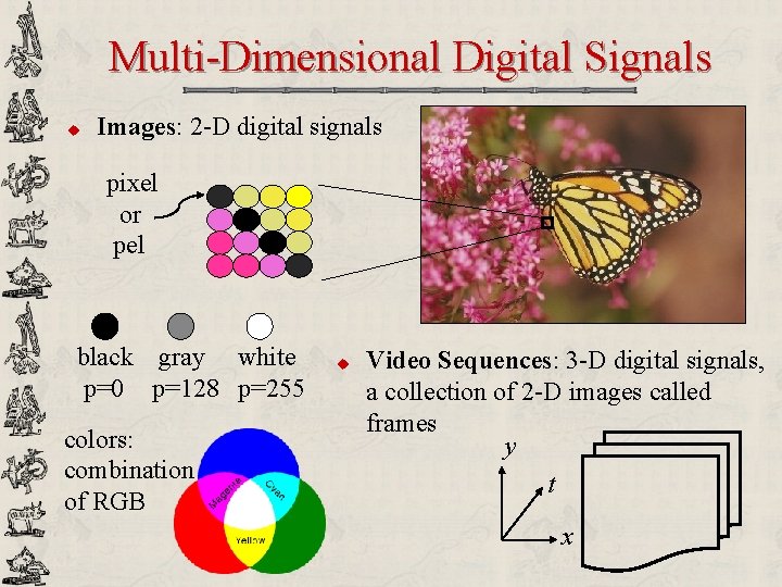
Multi-Dimensional Digital Signals u Images: 2 -D digital signals pixel or pel black gray white p=0 p=128 p=255 colors: combination of RGB u Video Sequences: 3 -D digital signals, a collection of 2 -D images called frames y t x

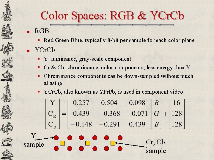
Color Spaces: RGB & YCr. Cb u RGB § Red Green Blue, typically 8 -bit per sample for each color plane u YCr. Cb § Y: luminance, gray-scale component § Cr & Cb: chrominance, color components, less energy than Y § Chrominance components can be down-sampled without much aliasing § YCr. Cb, also known as YPr. Pb, is used in component video Y sample Cr, Cb sample

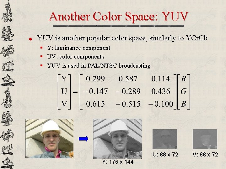
Another Color Space: YUV u YUV is another popular color space, similarly to YCr. Cb § Y: luminance component § UV: color components § YUV is used in PAL/NTSC broadcasting U: 88 x 72 Y: 176 x 144 V: 88 x 72

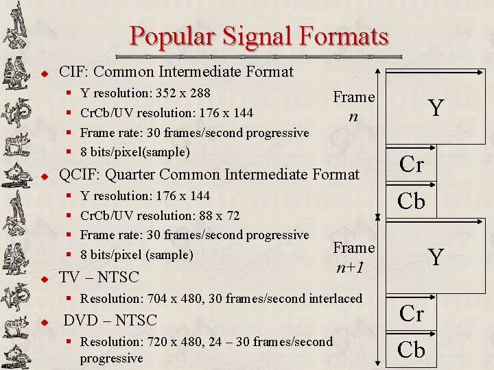
Popular Signal Formats u CIF: Common Intermediate Format § § u Frame n QCIF: Quarter Common Intermediate Format § § u Y resolution: 352 x 288 Cr. Cb/UV resolution: 176 x 144 Frame rate: 30 frames/second progressive 8 bits/pixel(sample) Y resolution: 176 x 144 Cr. Cb/UV resolution: 88 x 72 Frame rate: 30 frames/second progressive 8 bits/pixel (sample) TV – NTSC DVD – NTSC § Resolution: 720 x 480, 24 – 30 frames/second progressive Cr Cb Frame n+1 § Resolution: 704 x 480, 30 frames/second interlaced u Y Y Cr Cb

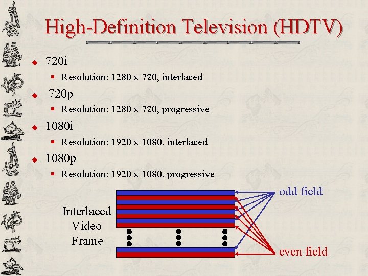
High-Definition Television (HDTV) u 720 i § Resolution: 1280 x 720, interlaced u 720 p § Resolution: 1280 x 720, progressive u 1080 i § Resolution: 1920 x 1080, interlaced u 1080 p § Resolution: 1920 x 1080, progressive odd field Interlaced Video Frame even field

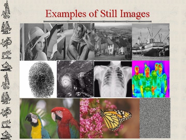
Examples of Still Images

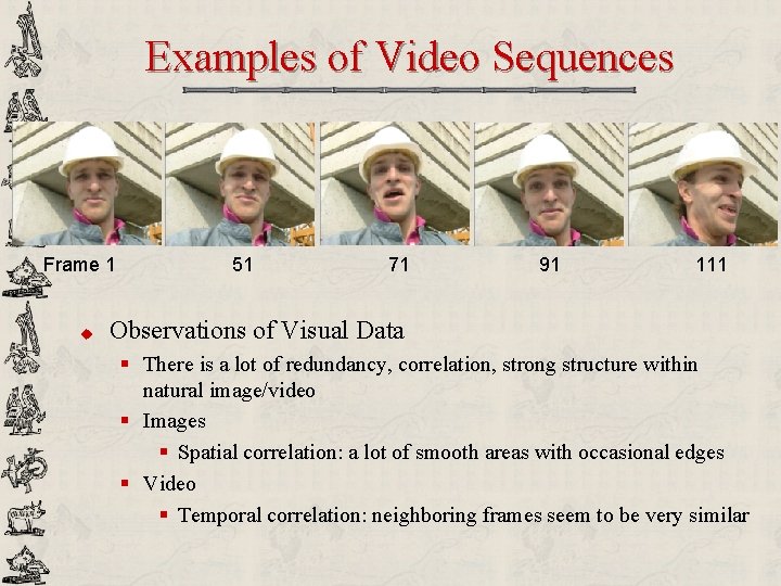
Examples of Video Sequences Frame 1 u 51 71 91 111 Observations of Visual Data § There is a lot of redundancy, correlation, strong structure within natural image/video § Images § Spatial correlation: a lot of smooth areas with occasional edges § Video § Temporal correlation: neighboring frames seem to be very similar

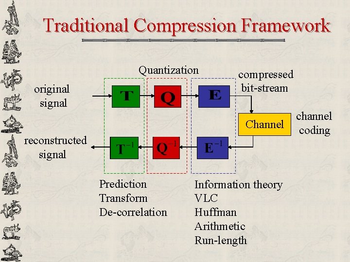
Traditional Compression Framework Quantization original signal compressed bit-stream Channel reconstructed signal Prediction Transform De-correlation Information theory VLC Huffman Arithmetic Run-length channel coding

Deterministic versus Random u Deterministic § Signals whose values can be specified explicitly § Example: a sinusoid u Random § Digital signals in practice can be treated as a collection of random variables or a random process § The symbols which occur randomly carry information u Probability theory § The study of random outcomes/events § Use mathematics to capture behavior of random outcomes and events

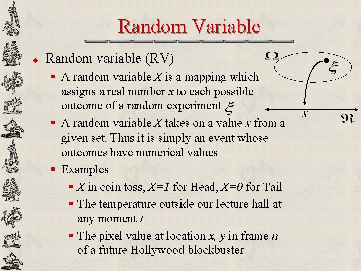
Random Variable u Random variable (RV) § A random variable X is a mapping which assigns a real number x to each possible outcome of a random experiment § A random variable X takes on a value x from a given set. Thus it is simply an event whose outcomes have numerical values § Examples § X in coin toss, X=1 for Head, X=0 for Tail § The temperature outside our lecture hall at any moment t § The pixel value at location x, y in frame n of a future Hollywood blockbuster x

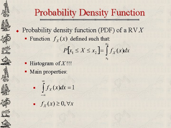
Probability Density Function u Probability density function (PDF) of a RV X § Function defined such that: § Histogram of X !!! § Main properties: § §

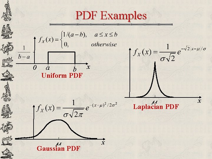
PDF Examples 0 a b x Uniform PDF Laplacian PDF Gaussian PDF x x

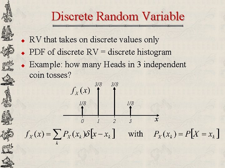
Discrete Random Variable u u u RV that takes on discrete values only PDF of discrete RV = discrete histogram Example: how many Heads in 3 independent coin tosses? 3/8 1/8 0 1/8 1 2 3 x

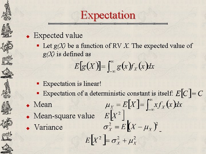
Expectation u Expected value § Let g(X) be a function of RV X. The expected value of g(X) is defined as § Expectation is linear! § Expectation of a deterministic constant is itself: u u u Mean-square value Variance

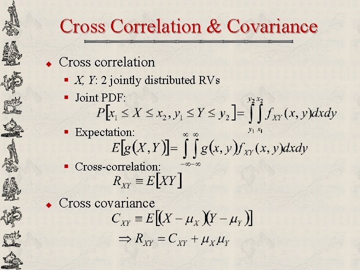
Cross Correlation & Covariance u Cross correlation § X, Y: 2 jointly distributed RVs § Joint PDF: § Expectation: § Cross-correlation: u Cross covariance

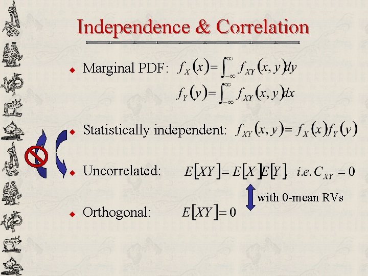
Independence & Correlation u Marginal PDF: u Statistically independent: u Uncorrelated: u Orthogonal: with 0 -mean RVs

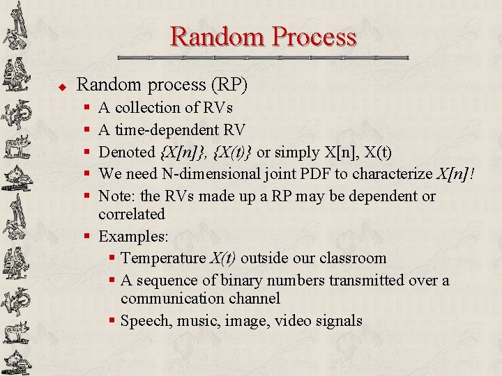
Random Process u Random process (RP) § § § A collection of RVs A time-dependent RV Denoted {X[n]}, {X(t)} or simply X[n], X(t) We need N-dimensional joint PDF to characterize X[n]! Note: the RVs made up a RP may be dependent or correlated § Examples: § Temperature X(t) outside our classroom § A sequence of binary numbers transmitted over a communication channel § Speech, music, image, video signals

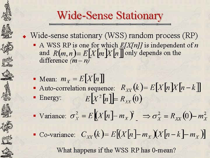
Wide-Sense Stationary u Wide-sense stationary (WSS) random process (RP) § A WSS RP is one for which E[X[n]] is independent of n and only depends on the difference (m – n) § Mean: § Auto-correlation sequence: § Energy: § Variance: § Co-variance: What happens if the WSS RP has 0 -mean?

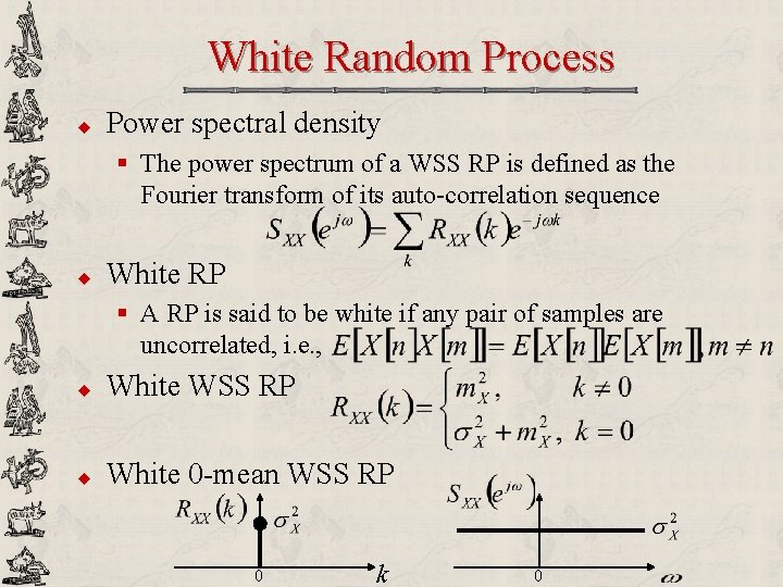
White Random Process u Power spectral density § The power spectrum of a WSS RP is defined as the Fourier transform of its auto-correlation sequence u White RP § A RP is said to be white if any pair of samples are uncorrelated, i. e. , u White WSS RP u White 0 -mean WSS RP 0 k 0

Stochastic Signal Model w[n] x[n] white 0 -mean WSS Gaussian noise u For speech: N = 10 to 20 u For images: N = 1! and AR(1) Signal AR(N) signal

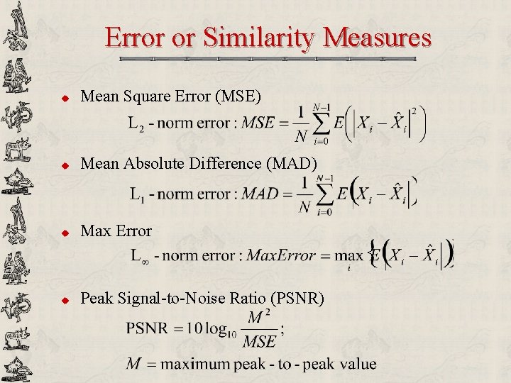
Error or Similarity Measures u Mean Square Error (MSE) u Mean Absolute Difference (MAD) u Max Error u Peak Signal-to-Noise Ratio (PSNR)

Summary u Introduction to natural signals § Natural digital signals are everywhere in our life § Efficient representation (compression) of digital signals facilitates information storage, archival, communications and even processing § Compression is achievable since visual data contains a lot of redundancy, both spatially and temporally u Review § § Random variables, PDF, mean, variance, correlation Random processes, wide-sense stationary RP, white Simple stochastic signal models via AR processes Error or similarity measures

Lossless Compression and Information Theory Trac D. Tran ECE Department The Johns Hopkins University Baltimore, MD 21218

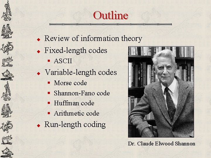
Outline u u Review of information theory Fixed-length codes § ASCII u Variable-length codes § § u Morse code Shannon-Fano code Huffman code Arithmetic code Run-length coding Dr. Claude Elwood Shannon

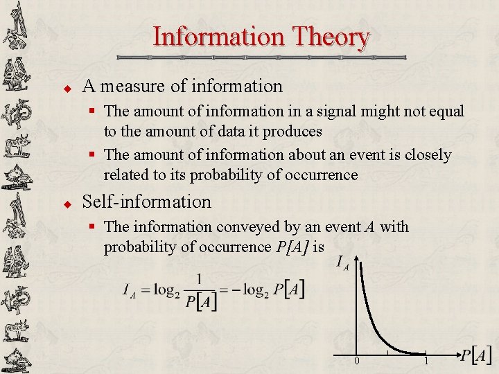
Information Theory u A measure of information § The amount of information in a signal might not equal to the amount of data it produces § The amount of information about an event is closely related to its probability of occurrence u Self-information § The information conveyed by an event A with probability of occurrence P[A] is 0 1

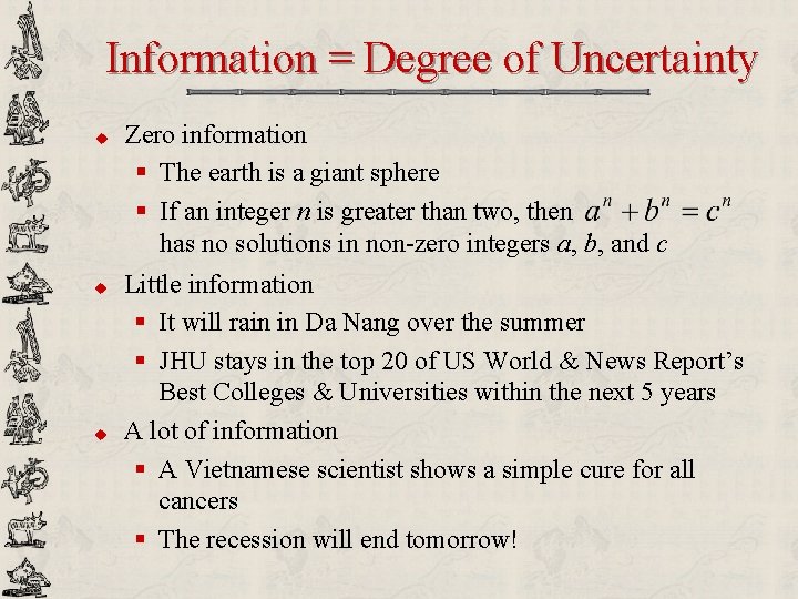
Information = Degree of Uncertainty u u u Zero information § The earth is a giant sphere § If an integer n is greater than two, then has no solutions in non-zero integers a, b, and c Little information § It will rain in Da Nang over the summer § JHU stays in the top 20 of US World & News Report’s Best Colleges & Universities within the next 5 years A lot of information § A Vietnamese scientist shows a simple cure for all cancers § The recession will end tomorrow!

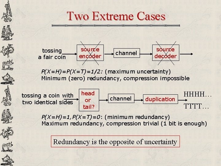
Two Extreme Cases tossing a fair coin source encoder channel source decoder P(X=H)=P(X=T)=1/2: (maximum uncertainty) Minimum (zero) redundancy, compression impossible tossing a coin with two identical sides head or tail? channel duplication HHHH… TTTT… P(X=H)=1, P(X=T)=0: (minimum redundancy) Maximum redundancy, compression trivial (1 bit is enough) Redundancy is the opposite of uncertainty

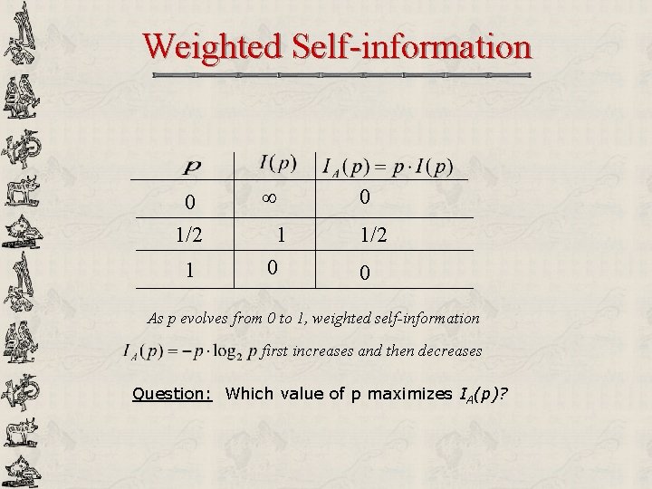
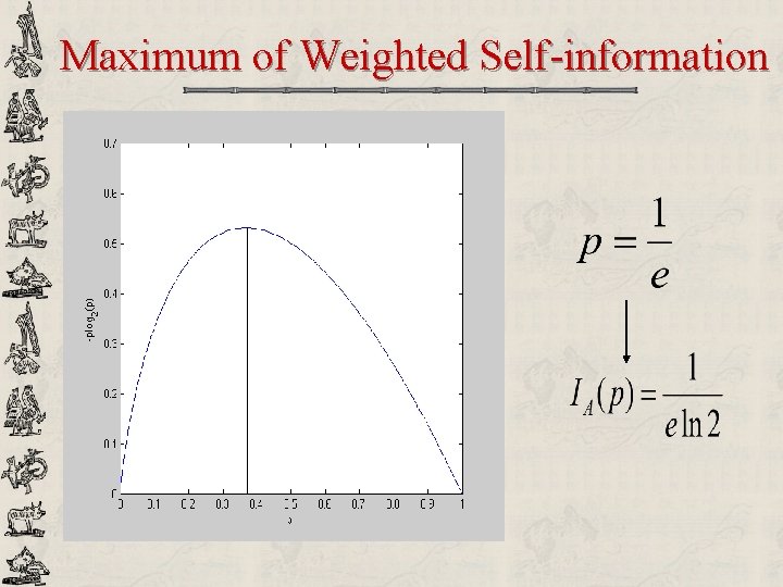
Weighted Self-information 0 1/2 1 0 1/2 0 As p evolves from 0 to 1, weighted self-information first increases and then decreases Question: Which value of p maximizes IA(p)?

Maximum of Weighted Self-information

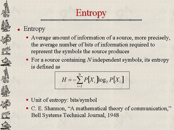
Entropy u Entropy § Average amount of information of a source, more precisely, the average number of bits of information required to represent the symbols the source produces § For a source containing N independent symbols, its entropy is defined as § Unit of entropy: bits/symbol § C. E. Shannon, “A mathematical theory of communication, ” Bell Systems Technical Journal, 1948

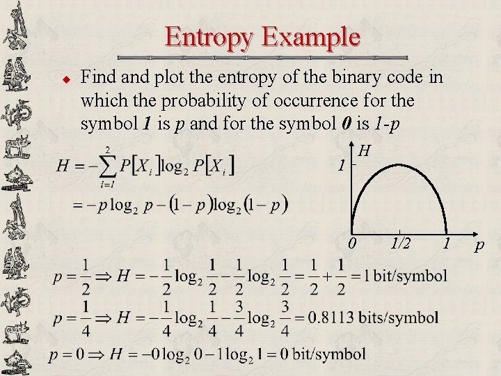
Entropy Example u Find and plot the entropy of the binary code in which the probability of occurrence for the symbol 1 is p and for the symbol 0 is 1 -p H 1 0 1/2 1 p

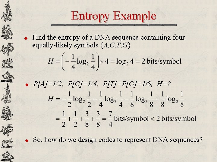
Entropy Example u Find the entropy of a DNA sequence containing four equally-likely symbols {A, C, T, G} u P[A]=1/2; P[C]=1/4; P[T]=P[G]=1/8; H=? u So, how do we design codes to represent DNA sequences?

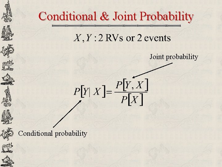
Conditional & Joint Probability Joint probability Conditional probability

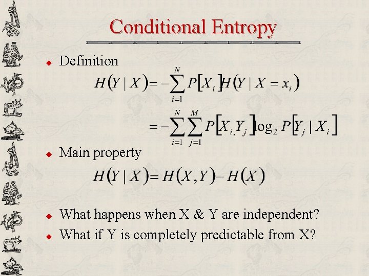
Conditional Entropy u Definition u Main property u u What happens when X & Y are independent? What if Y is completely predictable from X?

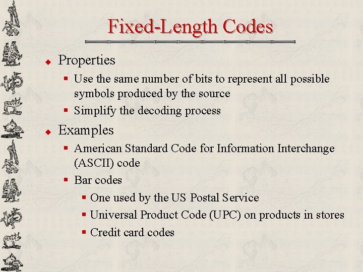
Fixed-Length Codes u Properties § Use the same number of bits to represent all possible symbols produced by the source § Simplify the decoding process u Examples § American Standard Code for Information Interchange (ASCII) code § Bar codes § One used by the US Postal Service § Universal Product Code (UPC) on products in stores § Credit card codes

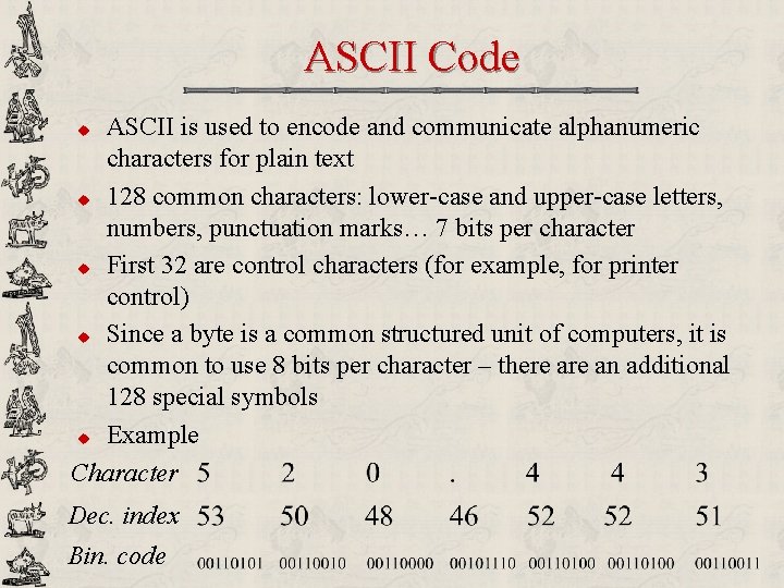
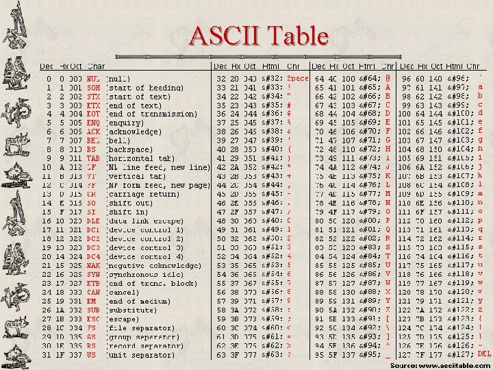
ASCII Code ASCII is used to encode and communicate alphanumeric characters for plain text u 128 common characters: lower-case and upper-case letters, numbers, punctuation marks… 7 bits per character u First 32 are control characters (for example, for printer control) u Since a byte is a common structured unit of computers, it is common to use 8 bits per character – there an additional 128 special symbols u Example Character u Dec. index Bin. code

ASCII Table

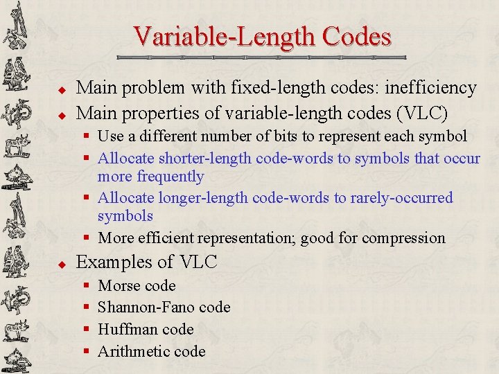
Variable-Length Codes u u Main problem with fixed-length codes: inefficiency Main properties of variable-length codes (VLC) § Use a different number of bits to represent each symbol § Allocate shorter-length code-words to symbols that occur more frequently § Allocate longer-length code-words to rarely-occurred symbols § More efficient representation; good for compression u Examples of VLC § § Morse code Shannon-Fano code Huffman code Arithmetic code

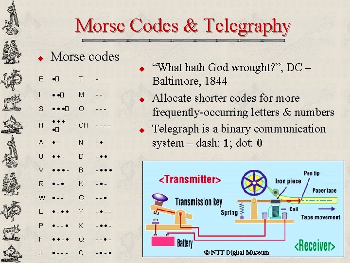
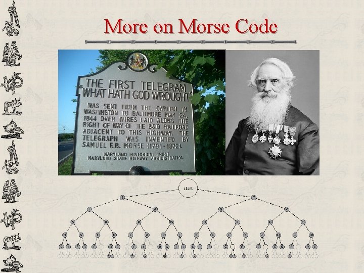
Morse Codes & Telegraphy u Morse codes u E ·� T - I · ·� M -- S · · ·� O --- H ··· ·� CH ---- A ·- N -· U ··- D -·· V ···- B -··· R ·-· K -·- W ·-- G --· L ·-·· Y -·-- P ·--· X -··- F ··-· Q --·- J ·--- C -·-· u u “What hath God wrought? ”, DC – Baltimore, 1844 Allocate shorter codes for more frequently-occurring letters & numbers Telegraph is a binary communication system – dash: 1; dot: 0

More on Morse Code

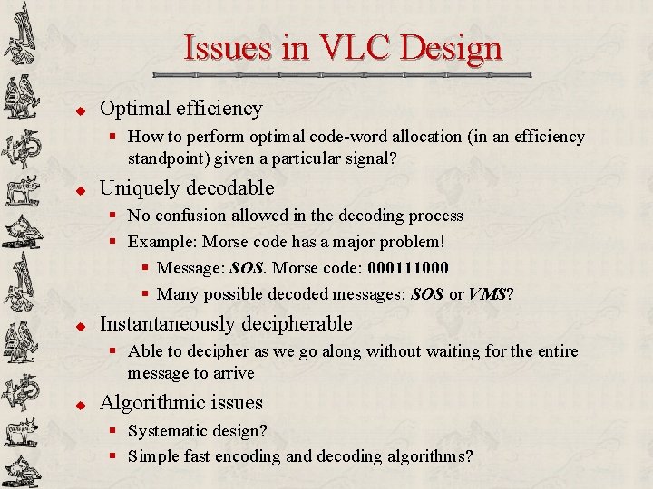
Issues in VLC Design u Optimal efficiency § How to perform optimal code-word allocation (in an efficiency standpoint) given a particular signal? u Uniquely decodable § No confusion allowed in the decoding process § Example: Morse code has a major problem! § Message: SOS. Morse code: 000111000 § Many possible decoded messages: SOS or VMS? u Instantaneously decipherable § Able to decipher as we go along without waiting for the entire message to arrive u Algorithmic issues § Systematic design? § Simple fast encoding and decoding algorithms?

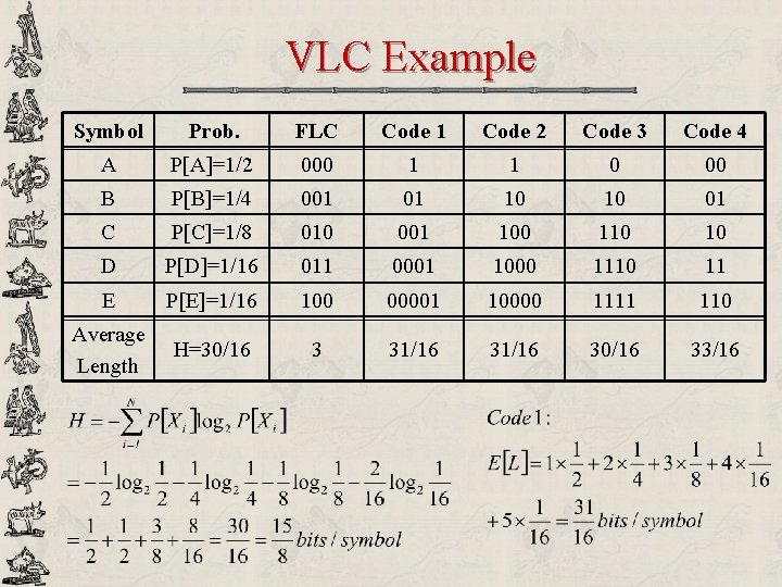
VLC Example Symbol Prob. FLC Code 1 Code 2 Code 3 Code 4 A P[A]=1/2 000 1 1 0 00 B P[B]=1/4 001 01 10 10 01 C P[C]=1/8 010 001 100 110 10 D P[D]=1/16 011 0001 1000 1110 11 E P[E]=1/16 100 00001 10000 1111 110 Average Length H=30/16 3 31/16 30/16 33/16

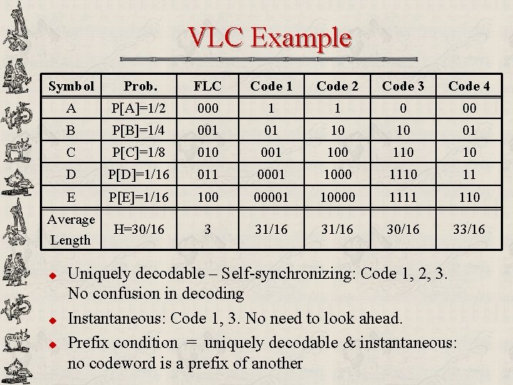
VLC Example Symbol Prob. FLC Code 1 Code 2 Code 3 Code 4 A P[A]=1/2 000 1 1 0 00 B P[B]=1/4 001 01 10 10 01 C P[C]=1/8 010 001 100 110 10 D P[D]=1/16 011 0001 1000 1110 11 E P[E]=1/16 100 00001 10000 1111 110 Average Length H=30/16 3 31/16 30/16 33/16 u u u Uniquely decodable – Self-synchronizing: Code 1, 2, 3. No confusion in decoding Instantaneous: Code 1, 3. No need to look ahead. Prefix condition = uniquely decodable & instantaneous: no codeword is a prefix of another

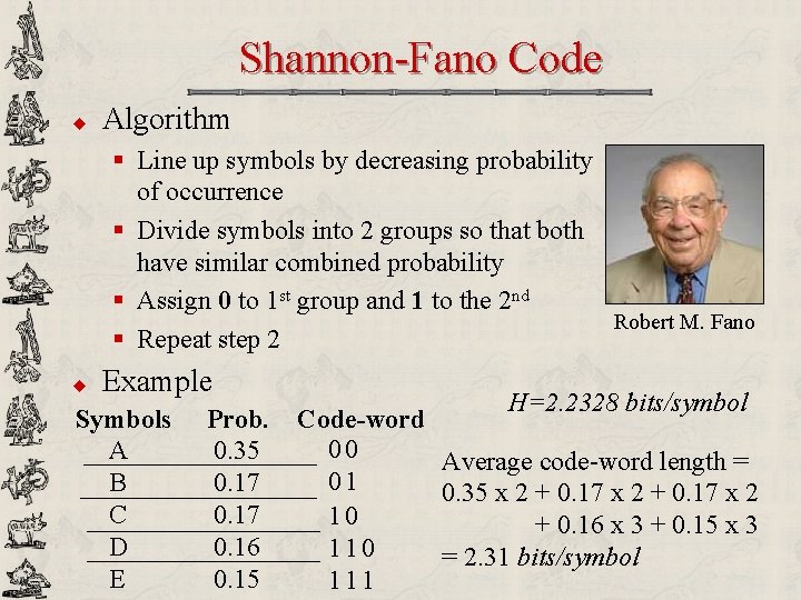
Shannon-Fano Code u Algorithm § Line up symbols by decreasing probability of occurrence § Divide symbols into 2 groups so that both have similar combined probability § Assign 0 to 1 st group and 1 to the 2 nd Robert M. Fano § Repeat step 2 u Example Symbols A B C D E Prob. 0. 35 0. 17 0. 16 0. 15 H=2. 2328 bits/symbol Code-word 00 Average code-word length = 01 0. 35 x 2 + 0. 17 x 2 10 + 0. 16 x 3 + 0. 15 x 3 110 = 2. 31 bits/symbol 111

Huffman Code u Shannon-Fano code [1949] § Top-down algorithm: assigning code from most frequent to least frequent § VLC, uniquely & instantaneously decodable (no code-word is a prefix of another) § Unfortunately not optimal in term of minimum redundancy u Huffman code [1952] § Quite similar to Shannon-Fano in VLC David A. Huffman concept § Bottom-up algorithm: assigning code from least frequent to most frequent § Minimum redundancy when probabilities of occurrence are powers-of-two § In JPEG images, DVD movies, MP 3 music

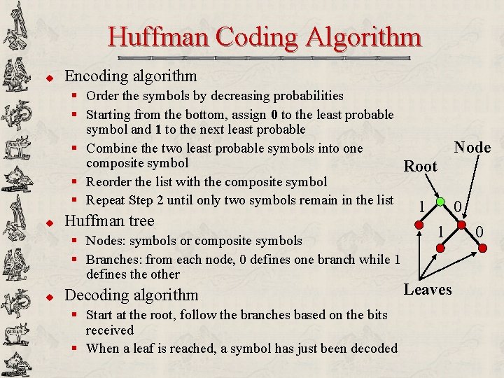
Huffman Coding Algorithm u Encoding algorithm § Order the symbols by decreasing probabilities § Starting from the bottom, assign 0 to the least probable symbol and 1 to the next least probable § Combine the two least probable symbols into one composite symbol Root § Reorder the list with the composite symbol § Repeat Step 2 until only two symbols remain in the list u Huffman tree § Nodes: symbols or composite symbols § Branches: from each node, 0 defines one branch while 1 defines the other u Decoding algorithm § Start at the root, follow the branches based on the bits received § When a leaf is reached, a symbol has just been decoded 1 1 Leaves Node 0 0

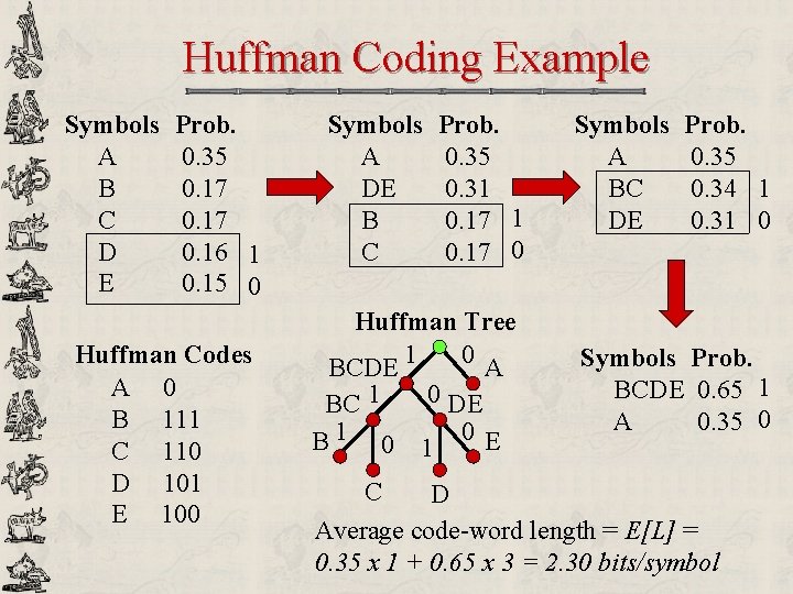
Huffman Coding Example Symbols A B C D E Prob. 0. 35 0. 17 0. 16 1 0. 15 0 Huffman Codes A 0 B 111 C 110 D 101 E 100 Symbols A DE B C Prob. 0. 35 0. 31 0. 17 0 Huffman Tree 1 0 BCDE A 0 DE BC 1 B 1 0 E Symbols A BC DE Prob. 0. 35 0. 34 1 0. 31 0 Symbols Prob. BCDE 0. 65 1 A 0. 35 0 C D Average code-word length = E[L] = 0. 35 x 1 + 0. 65 x 3 = 2. 30 bits/symbol

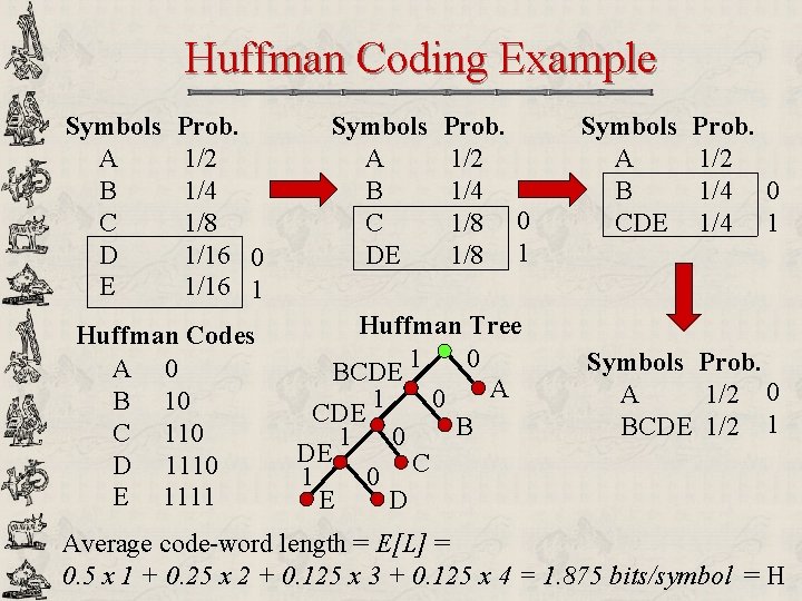
Huffman Coding Example Symbols A B C D E Prob. 1/2 1/4 1/8 1/16 0 1/16 1 Huffman Codes A 0 B 10 C 110 D 1110 E 1111 Symbols A B C DE Prob. 1/2 1/4 1/8 0 1/8 1 Huffman Tree 1 0 BCDE A 1 0 CDE B 1 0 DE C 1 0 D E Symbols A B CDE Prob. 1/2 1/4 0 1/4 1 Symbols Prob. A 1/2 0 BCDE 1/2 1 Average code-word length = E[L] = 0. 5 x 1 + 0. 25 x 2 + 0. 125 x 3 + 0. 125 x 4 = 1. 875 bits/symbol = H

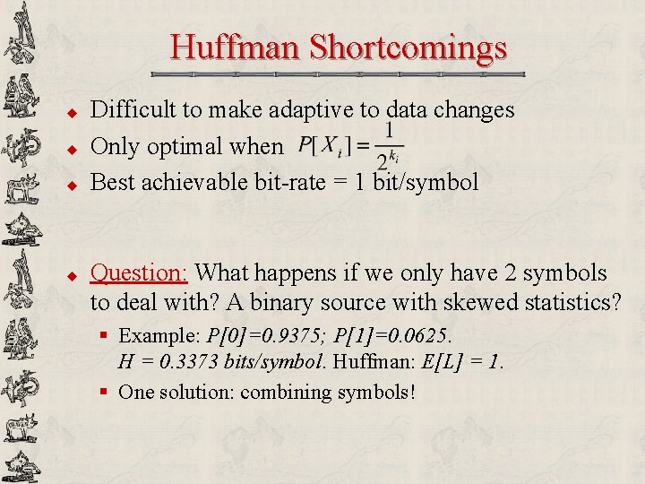
Huffman Shortcomings u u Difficult to make adaptive to data changes Only optimal when Best achievable bit-rate = 1 bit/symbol Question: What happens if we only have 2 symbols to deal with? A binary source with skewed statistics? § Example: P[0]=0. 9375; P[1]=0. 0625. H = 0. 3373 bits/symbol. Huffman: E[L] = 1. § One solution: combining symbols!

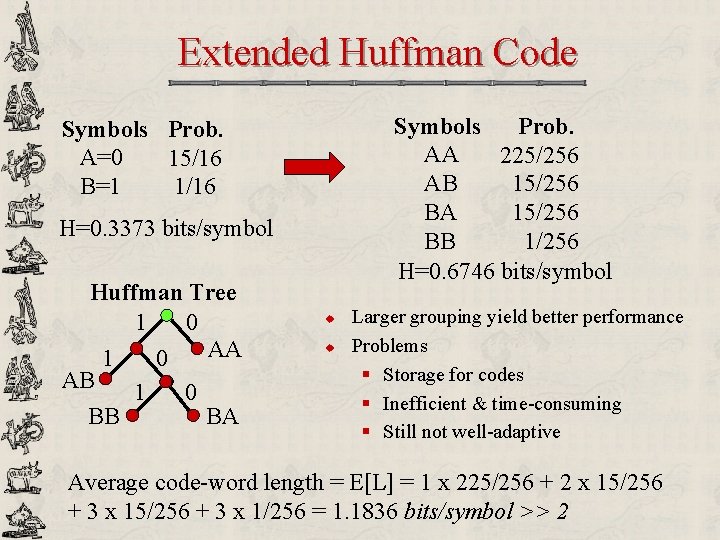
Extended Huffman Code Symbols Prob. AA 225/256 AB 15/256 BA 15/256 BB 1/256 H=0. 6746 bits/symbol Symbols Prob. A=0 15/16 B=1 1/16 H=0. 3373 bits/symbol Huffman Tree 1 0 AA 1 0 AB 1 0 BB BA u u Larger grouping yield better performance Problems § Storage for codes § Inefficient & time-consuming § Still not well-adaptive Average code-word length = E[L] = 1 x 225/256 + 2 x 15/256 + 3 x 1/256 = 1. 1836 bits/symbol >> 2

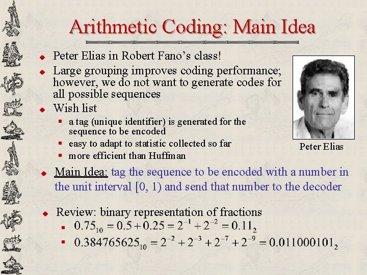
Arithmetic Coding: Main Idea u u u Peter Elias in Robert Fano’s class! Large grouping improves coding performance; however, we do not want to generate codes for all possible sequences Wish list § a tag (unique identifier) is generated for the sequence to be encoded § easy to adapt to statistic collected so far § more efficient than Huffman u u Peter Elias Main Idea: tag the sequence to be encoded with a number in the unit interval [0, 1) and send that number to the decoder Review: binary representation of fractions § §

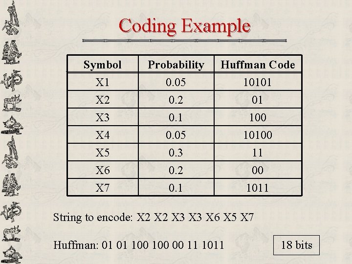
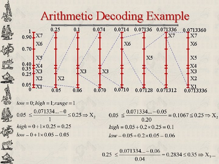
Coding Example Symbol X 1 X 2 X 3 Probability 0. 05 0. 2 0. 1 Huffman Code 10101 01 100 X 4 X 5 X 6 X 7 0. 05 0. 3 0. 2 0. 1 10100 11 00 1011 String to encode: X 2 X 3 X 6 X 5 X 7 Huffman: 01 01 100 00 11 1011 18 bits

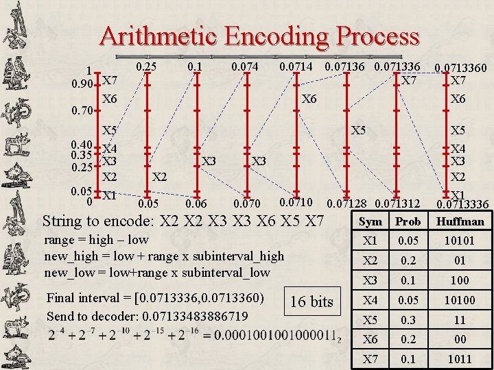
Arithmetic Encoding Process 1 0. 90 X 7 X 6 0. 70 0. 25 0. 1 0. 074 0. 07136 0. 071336 X 7 X 6 X 5 0. 40 X 4 0. 35 X 3 0. 25 X 2 0. 05 X 1 0 X 6 X 5 X 3 X 5 X 4 X 3 X 2 0. 05 0. 06 0. 070 0. 0710 String to encode: X 2 X 3 X 6 X 5 0. 07128 0. 071312 Sym Prob X 7 range = high – low new_high = low + range x subinterval_high new_low = low+range x subinterval_low Final interval = [0. 0713336, 0. 0713360) Send to decoder: 0. 07133483886719 0. 0713360 X 7 16 bits X 1 0. 0713336 Huffman X 1 0. 05 10101 X 2 01 X 3 0. 1 100 X 4 0. 05 10100 X 5 0. 3 11 X 6 0. 2 00 X 7 0. 1 1011

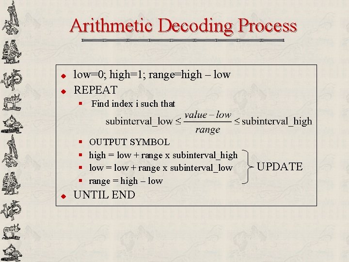
Arithmetic Decoding Process u u low=0; high=1; range=high – low REPEAT § Find index i such that § § u OUTPUT SYMBOL high = low + range x subinterval_high low = low + range x subinterval_low range = high – low UNTIL END UPDATE

Arithmetic Decoding Example 1 0. 90 X 7 X 6 0. 70 0. 25 0. 1 0. 074 0. 07136 0. 071336 X 7 X 6 X 5 0. 40 X 4 0. 35 X 3 0. 25 X 2 0. 05 X 1 0 X 6 X 5 X 3 0. 06 X 3 0. 070 X 5 X 4 X 3 X 2 0. 05 0. 0713360 X 7 0. 0710 0. 07128 0. 071312 X 1 0. 0713336

Adaptive Arithmetic Coding u Three symbols {A, B, C}. Encode: BCCB… 1 P[C]=1/3 66% 0. 666 75% 33% P[A]=1/3 0 P[C]=1/4 P[B]=1/2 P[B]=1/3 25% 0. 666 P[C]=2/5 A B P[C]=1/2 60% P[B]=2/5 P[A]=1/4 20% 0. 333 0. 666 P[A]=1/5 0. 5834 Final interval = [0. 6390, 0. 6501) 50% P[B]=1/3 16% P[A]=1/6 0. 6334 Decode? C

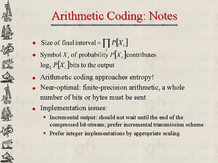
Arithmetic Coding: Notes u u u Arithmetic coding approaches entropy! Near-optimal: finite-precision arithmetic, a whole number of bits or bytes must be sent Implementation issues: § Incremental output: should not wait until the end of the compressed bit-stream; prefer incremental transmission scheme § Prefer integer implementations by appropriate scaling

Run-Length Coding u Main idea § Encoding long runs of a single symbol by the length of the run u Properties § A lossless coding scheme § Our first attempt at inter-symbol coding § Really effective with transform-based coding since the transform usually produces long runs of insignificant coefficients § Run-length coding can be combined with other entropy coding techniques (for example, run-length and Huffman coding in JPEG)

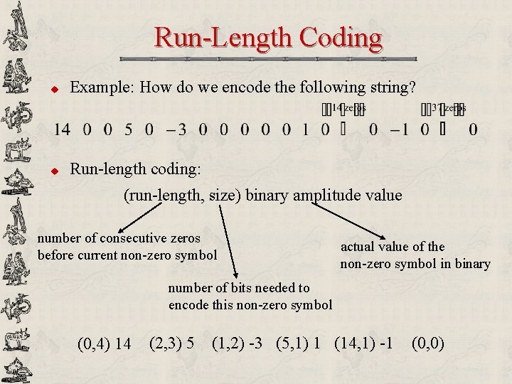
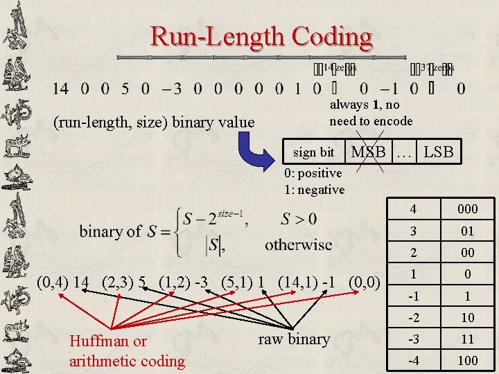
Run-Length Coding u Example: How do we encode the following string? u Run-length coding: (run-length, size) binary amplitude value number of consecutive zeros before current non-zero symbol actual value of the non-zero symbol in binary number of bits needed to encode this non-zero symbol (0, 4) 14 (2, 3) 5 (1, 2) -3 (5, 1) 1 (14, 1) -1 (0, 0)

Run-Length Coding (run-length, size) binary value always 1, no need to encode sign bit 0: positive 1: negative MSB … LSB (0, 4) 14 (2, 3) 5 (1, 2) -3 (5, 1) 1 (14, 1) -1 (0, 0) Huffman or arithmetic coding raw binary 4 000 3 01 2 00 1 0 -1 1 -2 10 -3 11 -4 100

Lossy Compression and Quantization Trac D. Tran ECE Department The Johns Hopkins University Baltimore, MD 21218

Outline u u Review Quantization § Nonlinear mapping § Forward and inverse quantization § Quantization errors § Clipping error § Approximation error § Error model § Optimal scalar quantization § Examples

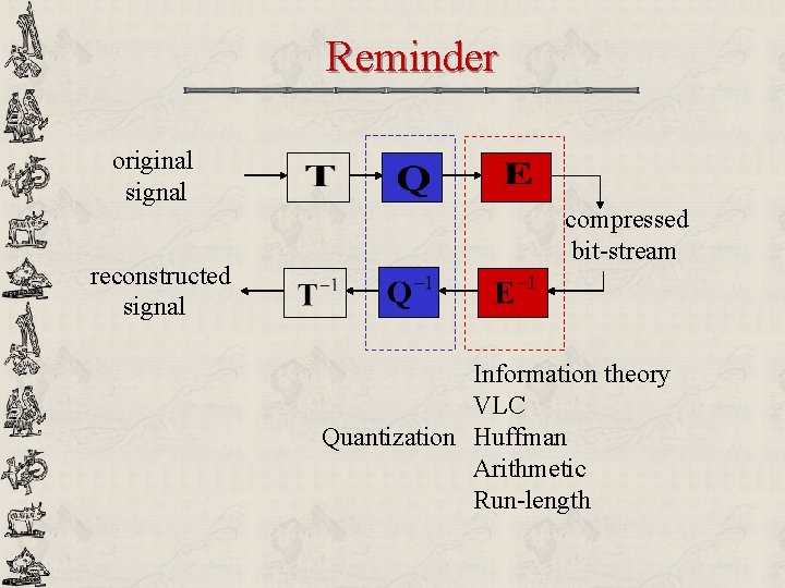
Reminder original signal reconstructed signal compressed bit-stream Information theory VLC Quantization Huffman Arithmetic Run-length

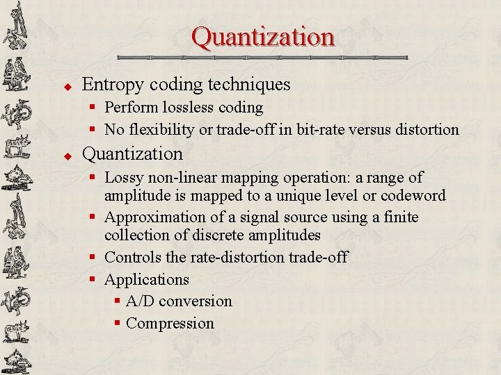
Quantization u Entropy coding techniques § Perform lossless coding § No flexibility or trade-off in bit-rate versus distortion u Quantization § Lossy non-linear mapping operation: a range of amplitude is mapped to a unique level or codeword § Approximation of a signal source using a finite collection of discrete amplitudes § Controls the rate-distortion trade-off § Applications § A/D conversion § Compression

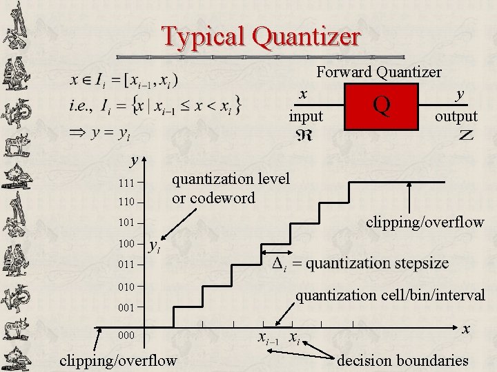
Typical Quantizer Forward Quantizer x input Q y output y 111 110 quantization level or codeword 101 clipping/overflow 100 011 010 001 000 clipping/overflow quantization cell/bin/interval x decision boundaries

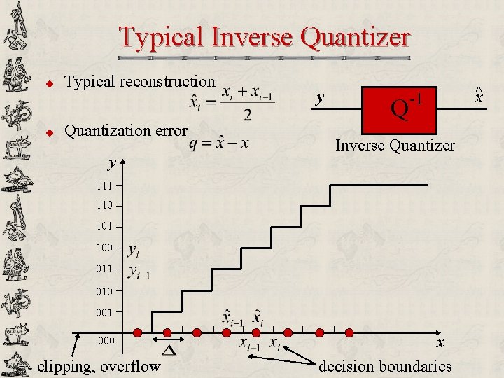
Typical Inverse Quantizer u u Typical reconstruction Quantization error y y Q -1 Inverse Quantizer 111 110 101 100 011 010 001 000 clipping, overflow x decision boundaries ^x

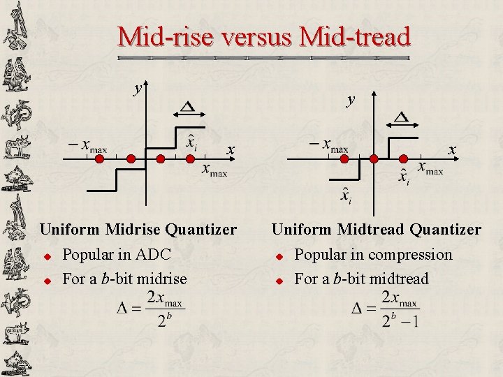
Mid-rise versus Mid-tread y y x Uniform Midrise Quantizer u u Popular in ADC For a b-bit midrise x Uniform Midtread Quantizer u u Popular in compression For a b-bit midtread

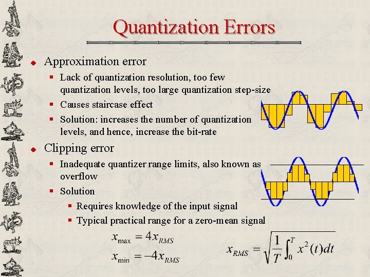
Quantization Errors u Approximation error § Lack of quantization resolution, too few quantization levels, too large quantization step-size § Causes staircase effect § Solution: increases the number of quantization levels, and hence, increase the bit-rate u Clipping error § Inadequate quantizer range limits, also known as overflow § Solution § Requires knowledge of the input signal § Typical practical range for a zero-mean signal

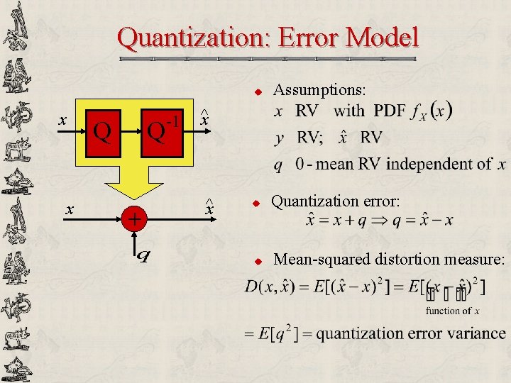
Quantization: Error Model x x Q Q + -1 u Assumptions: u Quantization error: u Mean-squared distortion measure: ^x x^

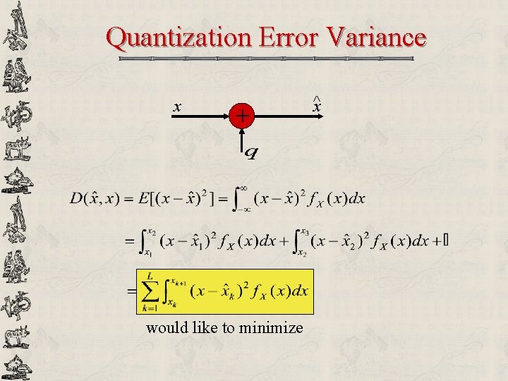
Quantization Error Variance x + would like to minimize ^x

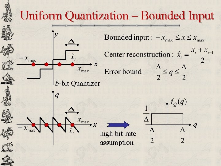
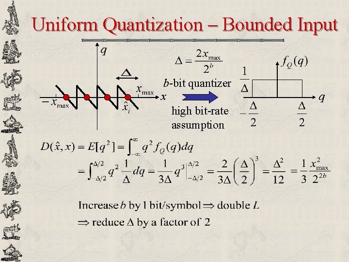
Uniform Quantization – Bounded Input y x b-bit Quantizer q x q high bit-rate assumption

Uniform Quantization – Bounded Input q b-bit quantizer x high bit-rate assumption q

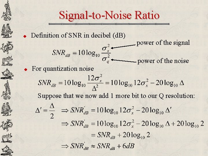
Signal-to-Noise Ratio u Definition of SNR in decibel (d. B) power of the signal power of the noise u For quantization noise Suppose that we now add 1 more bit to our Q resolution:

Example Design a 3 -bit uniform quantizer for a signal with range [0, 128] u Maximum possible number of levels: u Quantization stepsize: u Quantization levels: u Reconstruction levels: u Maximum quantization error:

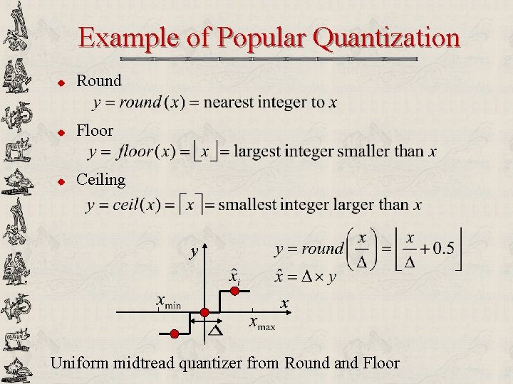
Example of Popular Quantization u Round u Floor u Ceiling y x Uniform midtread quantizer from Round and Floor

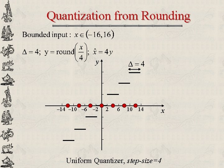
Quantization from Rounding y – 14 – 10 – 6 – 2 2 6 10 14 x Uniform Quantizer, step-size=4

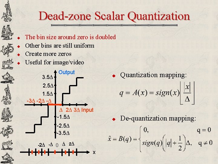
Dead-zone Scalar Quantization u u The bin size around zero is doubled Other bins are still uniform Create more zeros Useful for image/video 3. 5∆ Output u Quantization mapping: u De-quantization mapping: 2. 5∆ 1. 5∆ -3∆ -2∆ -∆ ∆ 2∆ 3∆ Input -1. 5∆ -2. 5∆ -3. 5∆ -2∆ -∆ 0 ∆ 2∆ x

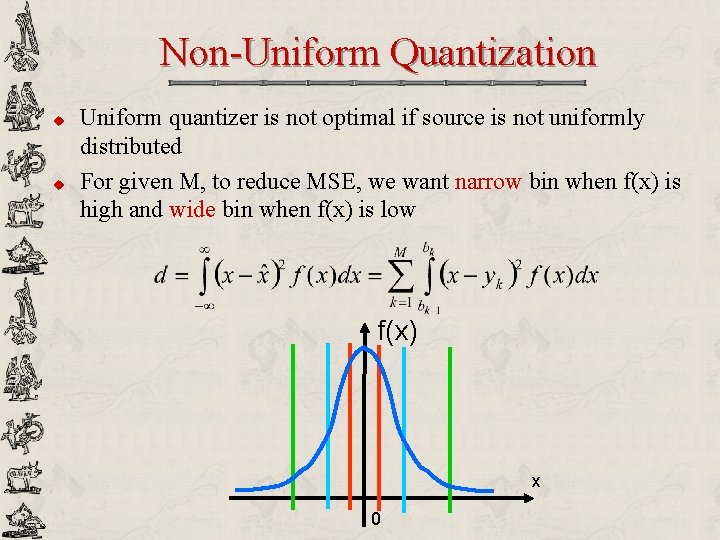
Non-Uniform Quantization u u Uniform quantizer is not optimal if source is not uniformly distributed For given M, to reduce MSE, we want narrow bin when f(x) is high and wide bin when f(x) is low f(x) x 0

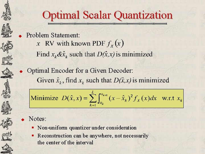
Optimal Scalar Quantization u Problem Statement: u Optimal Encoder for a Given Decoder: u Notes: § Non-uniform quantizer under consideration § Reconstruction can be anywhere, not necessarily the center of the interval

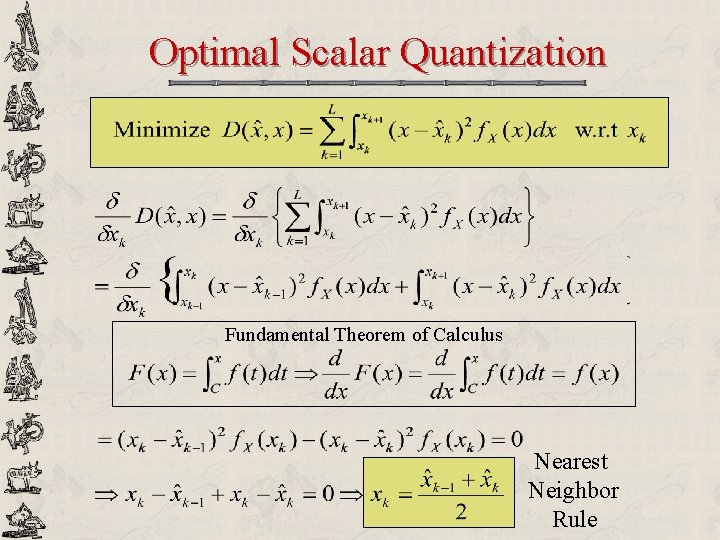
Optimal Scalar Quantization Fundamental Theorem of Calculus Nearest Neighbor Rule

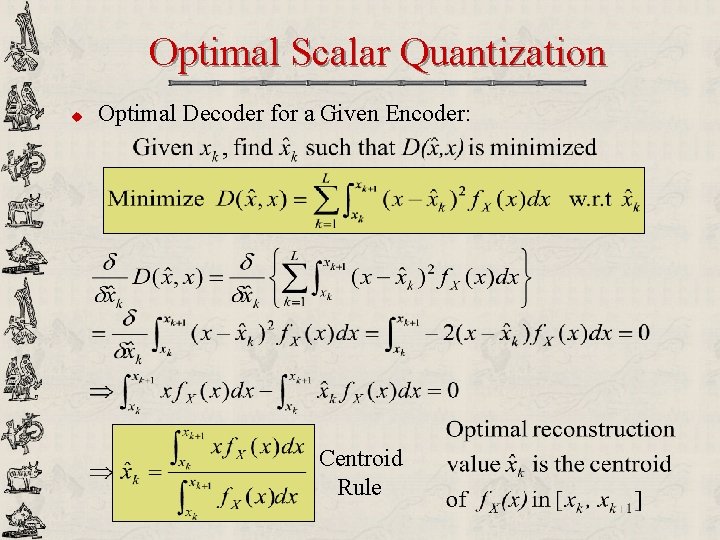
Optimal Scalar Quantization u Optimal Decoder for a Given Encoder: Centroid Rule

Lloyd-Max Quantizer u u Main idea [Lloyd 1957] [Max 1960] § solving these 2 equation iteratively until D converges Input Codebook Nearest Neighbor Partitioning Centroid Computation index of m-th iteration u Assumptions § Input PDF is known and stationary § Entropy has not been taken into account Updated Codebook

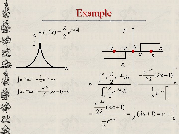
Example y –b x –a 0 a x b

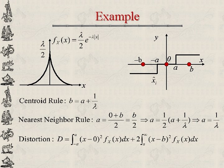
Example y –b x –a 0 a x b

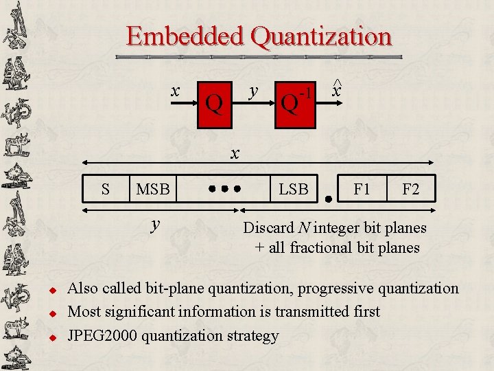
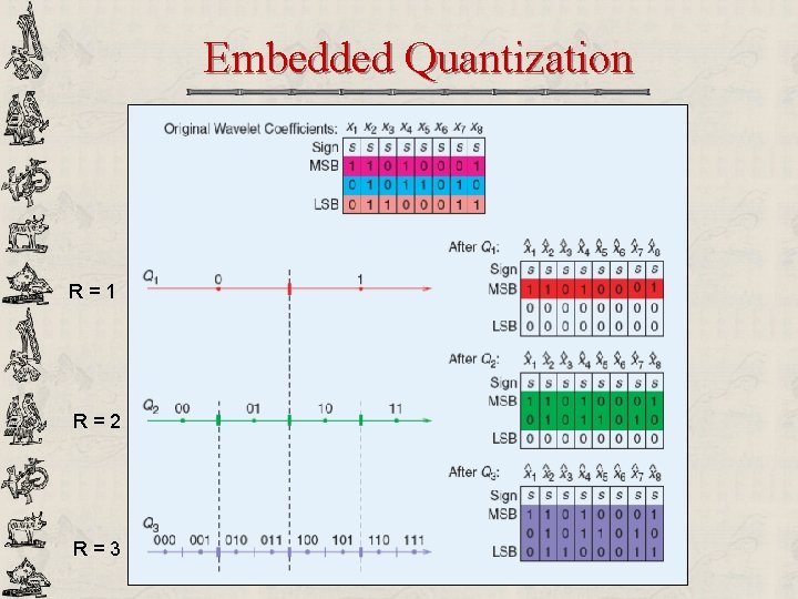
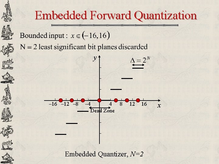
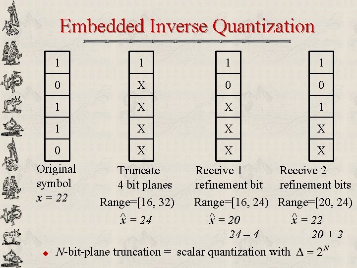
Embedded Quantization x y Q Q -1 ^x x S MSB y u u u LSB F 1 F 2 Discard N integer bit planes + all fractional bit planes Also called bit-plane quantization, progressive quantization Most significant information is transmitted first JPEG 2000 quantization strategy

Embedded Quantization R=1 R=2 R=3

Embedded Forward Quantization y – 16 – 12 – 8 – 4 4 8 Dead Zone 12 16 Embedded Quantizer, N=2 x

Embedded Inverse Quantization 1 1 0 X 0 0 1 X X 1 1 X X X 0 X X X Original symbol x = 22 u Truncate 4 bit planes Range=[16, 32) ^x = 24 Receive 1 Receive 2 refinement bits Range=[16, 24) Range=[20, 24) x^ = 20 x^ = 22 = 24 – 4 = 20 + 2 N-bit-plane truncation = scalar quantization with

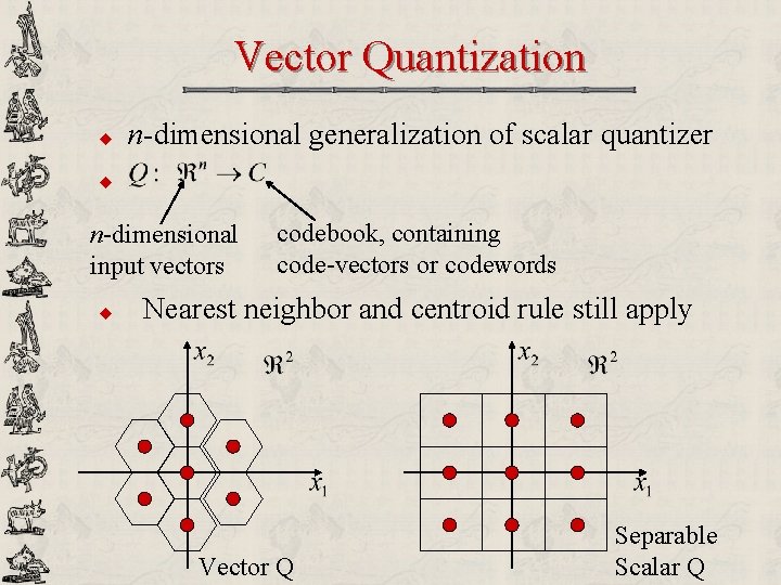
Vector Quantization u n-dimensional generalization of scalar quantizer u n-dimensional input vectors u codebook, containing code-vectors or codewords Nearest neighbor and centroid rule still apply Vector Q Separable Scalar Q

Summary u Introduction to audio/image/video signals § Sparsity in most signals facilitates information storage, archival, communications and even processing § Compression is achievable since naturally collected data contains a lot of redundancy, both spatially and temporally u Variable-length coding § Provides effective lossless coding capability § Huffman coding & arithmetic coding achieve bit rates close to entropy – the lowest achievable bit rate u Quantization § Allows lossy signal coding and aggressive compression § Provides trade-off between bit rate and reconstruction quality