Sparse Matrix Vector Multiply Algorithms and Optimizations on

Sparse Matrix Vector Multiply Algorithms and Optimizations on Modern Architectures Ankit Jain, Vasily Volkov CS 252 Final Presentation 5/9/2007 ankit@eecs. berkeley. edu volkov@eecs. berkeley. edu

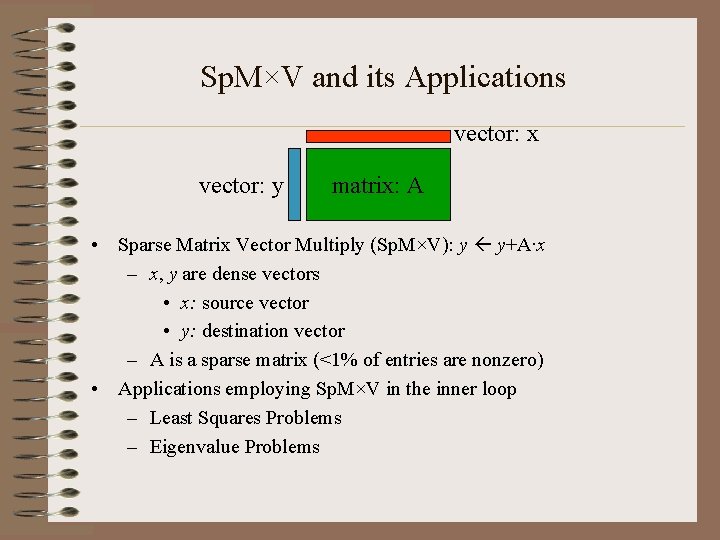
Sp. M×V and its Applications vector: x vector: y matrix: A • Sparse Matrix Vector Multiply (Sp. M×V): y y+A∙x – x, y are dense vectors • x: source vector • y: destination vector – A is a sparse matrix (<1% of entries are nonzero) • Applications employing Sp. M×V in the inner loop – Least Squares Problems – Eigenvalue Problems

Storing a Matrix in Memory type val : real[k] type ind : int[k] type ptr : int[m+1] 1 2 3 foreach row i do for l = ptr[i] to ptr[i + 1] – 1 do y[i] + val[l] ∙ x[ind[l]] Compressed Sparse Row Data Structure and Algorithm

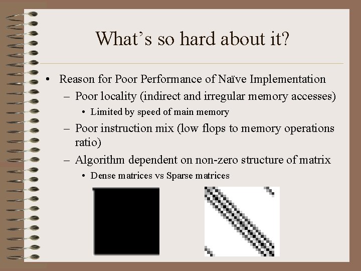
What’s so hard about it? • Reason for Poor Performance of Naïve Implementation – Poor locality (indirect and irregular memory accesses) • Limited by speed of main memory – Poor instruction mix (low flops to memory operations ratio) – Algorithm dependent on non-zero structure of matrix • Dense matrices vs Sparse matrices

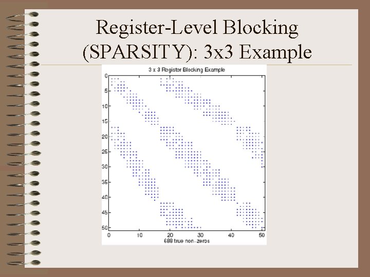
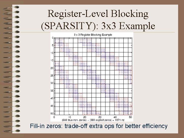
Register-Level Blocking (SPARSITY): 3 x 3 Example

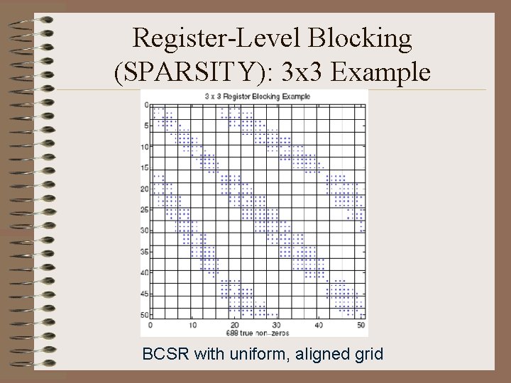
Register-Level Blocking (SPARSITY): 3 x 3 Example BCSR with uniform, aligned grid

Register-Level Blocking (SPARSITY): 3 x 3 Example Fill-in zeros: trade-off extra ops for better efficiency

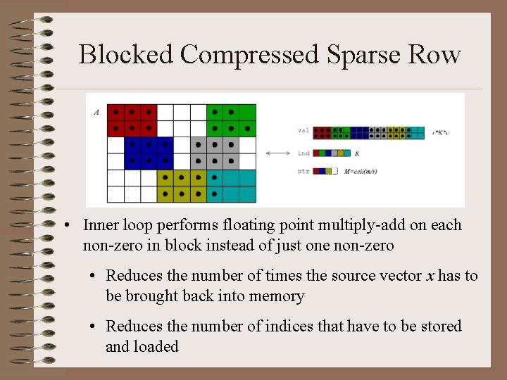
Blocked Compressed Sparse Row • Inner loop performs floating point multiply-add on each non-zero in block instead of just one non-zero • Reduces the number of times the source vector x has to be brought back into memory • Reduces the number of indices that have to be stored and loaded

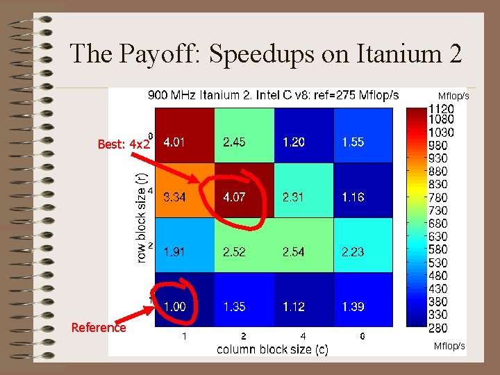
The Payoff: Speedups on Itanium 2 Mflop/s Best: 4 x 2 Reference Mflop/s

Explicit Software Pipelining ORIGINAL CODE: SOFTWARE PIPELINED CODE type val : real[k] type ind : int[k] type ptr : int[m+1] 1 2 3 foreach row i do for l = ptr[i] to ptr[i + 1] – 1 do type val : real[k] type ind : int[k] type ptr : int[m+1] 1 2 y[i] + val[l] ∙ x[ind[l]] 3 foreach row i do for l = ptr[i] to ptr[i + 1] – 1 do y[i] + val_1 ∙ x_1 4 val_1 = val[l + 1] 5 x_1 = x[ind_2] 6 ind_2 = ind[l + 2]

Explicit Software Prefetching ORIGINAL CODE: SOFTWARE PREFETCHED CODE type val : real[k] type ind : int[k] type ptr : int[m+1] 1 2 3 foreach row i do for l = ptr[i] to ptr[i + 1] – 1 do type val : real[k] type ind : int[k] type ptr : int[m+1] 1 2 y[i] + val[l] ∙ x[ind[l]] 3 foreach row i do for l = ptr[i] to ptr[i + 1] – 1 do y[i] + val[l] ∙ x[ind[l]] 4 pref(NTA, pref_v_amt + &val[l]) 5 pref(NTA, pref_i_amt + &ind[l]) 6 pref(NONE, &x[ind[l+pref_x_amt]]) 7 *NTA refers to no temporal locality on all levels 8 *NONE refers to temporal locality on highest Level

Characteristics of Modern Architectures • High Set Associativity in Caches – 4 -way L 1, 8 -way L 2, 12 -way L 3 Itanium 2 • Multiple Load Store Units • Multiple Execution Units – Six Integer Execution Units on Itanium 2 – Two Floating Point Multiply-Add Execution Units in Itanium 2 Question: What if we broke the matrix into multiple streams of execution?

Parallel Sp. MV • Run different rows in different threads • Can do that on data parallel architectures (SIMD/VLIW, Itanium/GPU)? – What if rows have different length? – One row finishes, other are still running • Waiting threads keep processors idle – Can we avoid idleness? • Standard solution: Segmented scan

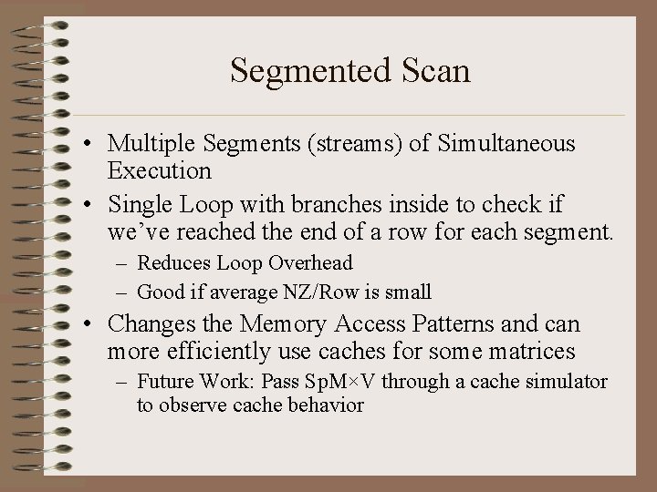
Segmented Scan • Multiple Segments (streams) of Simultaneous Execution • Single Loop with branches inside to check if we’ve reached the end of a row for each segment. – Reduces Loop Overhead – Good if average NZ/Row is small • Changes the Memory Access Patterns and can more efficiently use caches for some matrices – Future Work: Pass Sp. M×V through a cache simulator to observe cache behavior

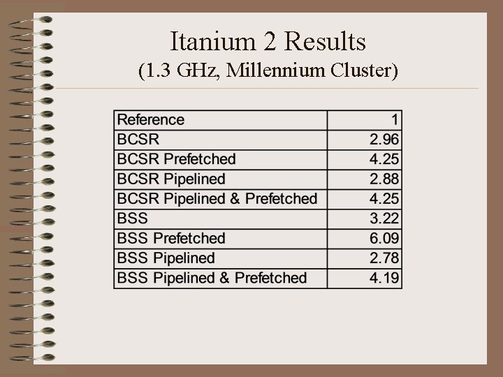
Itanium 2 Results (1. 3 GHz, Millennium Cluster)

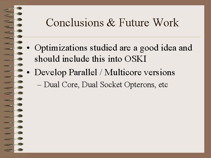
Conclusions & Future Work • Optimizations studied are a good idea and should include this into OSKI • Develop Parallel / Multicore versions – Dual Core, Dual Socket Opterons, etc

Questions?

Extra Slides

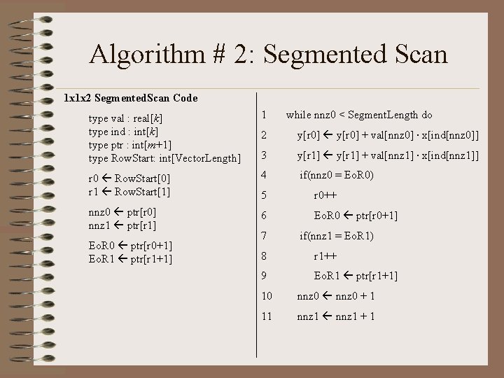
Algorithm # 2: Segmented Scan 1 x 1 x 2 Segmented. Scan Code type val : real[k] type ind : int[k] type ptr : int[m+1] type Row. Start: int[Vector. Length] 1 while nnz 0 < Segment. Length do 2 y[r 0] + val[nnz 0] ∙ x[ind[nnz 0]] 3 y[r 1] + val[nnz 1] ∙ x[ind[nnz 1]] r 0 Row. Start[0] r 1 Row. Start[1] 4 if(nnz 0 = Eo. R 0) 5 r 0++ nnz 0 ptr[r 0] nnz 1 ptr[r 1] 6 Eo. R 0 ptr[r 0+1] Eo. R 1 ptr[r 1+1] 8 r 1++ 9 Eo. R 1 ptr[r 1+1] 7 if(nnz 1 = Eo. R 1) 10 nnz 0 + 1 11 nnz 1 + 1

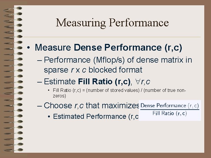
Measuring Performance • Measure Dense Performance (r, c) – Performance (Mflop/s) of dense matrix in sparse r x c blocked format – Estimate Fill Ratio (r, c), r, c • Fill Ratio (r, c) = (number of stored values) / (number of true nonzeros) – Choose r, c that maximizes • Estimated Performance (r, c) =

References 1. 2. 3. 4. 5. 6. 7. 8. G. Belloch, M. Heroux, and M. Zagha. Segmented operations for sparse matrix computation on vector multiprocessors. Technical Report CMU-CS-93 -173, Carnegie Mellon University, 1993. E. -J. Im. Optimizing the performance of sparse matrix-vector multiplication. Ph. D thesis, University of California, Berkeley, May 2000. E. -J. Im, K. A. Yelick, and R. Vuduc. SPARSITY: Framework for optimizing sparse matrixvector multiply. International Journal of High Performance Computing Applications, 18(1): 135 – 158, February 2004. R. Nishtala, R. W. Vuduc, J. W. Demmel, and K. A. Yelick. Performance Modeling and Analysis of Cache Blocking in Sparse Matrix Vector Multiply. Technical Report UCB/CSD-04 -1335, University of California, Berkeley, CA, USA, June 2004. Y. Saad. SPARSKIT: A basic tool kit for sparse matrix computations. Technical Report 90 -20, NASA Ames Research Center, Moffett Field, CA, 1990. A. Schwaighofer. A matlab interface to svm light to version 4. 0. http: //www. cis. tugraz. at/igi/aschwaig/software. html, 2004. R. Vuduc. Automatic Performance Tuning of Sparse Matrix Kernels. Ph. D thesis, University of California, Berkeley, December 2003. R. Vuduc, J. Demmel, and K. Yelick. OSKI: A library of automatically tuned sparse matrix kernels. In Proceedings of Sci. DAC 2005, Journal of Physics: Conference Series, San Francisco, CA, USA, June 2005. Institute of Physics Publishing. (to appear).