Spark SQL Relational Data Processing in Spark Michael

Spark SQL: Relational Data Processing in Spark Michael Armbrust, Reynold Xin, Cheng Lian, Yin Huai, Davies Liu, Joseph K. Bradley, Xiangrui Meng, Tomer Kaftan, Michael J. Franklin, Ali Ghodsi, Matei Zaharia SIGMOD 2015 – Melbourne, Australia Presented by Doris Xin Based on slides provided by M. Armbrust

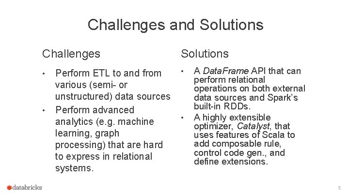
Challenges and Solutions Challenges • • Perform ETL to and from various (semi- or unstructured) data sources Perform advanced analytics (e. g. machine learning, graph processing) that are hard to express in relational systems. Solutions • • A Data. Frame API that can perform relational operations on both external data sources and Spark’s built-in RDDs. A highly extensible optimizer, Catalyst, that uses features of Scala to add composable rule, control code gen. , and define extensions. 2

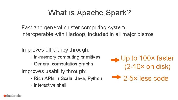
What is Apache Spark? Fast and general cluster computing system, interoperable with Hadoop, included in all major distros Improves efficiency through: • In-memory computing primitives • General computation graphs Improves usability through: • Rich APIs in Scala, Java, Python • Interactive shell Up to 100× faster (2 -10× on disk) 2 -5× less code

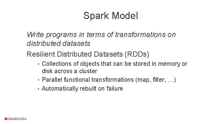
Spark Model Write programs in terms of transformations on distributed datasets Resilient Distributed Datasets (RDDs) • Collections of objects that can be stored in memory or disk across a cluster • Parallel functional transformations (map, filter, …) • Automatically rebuilt on failure

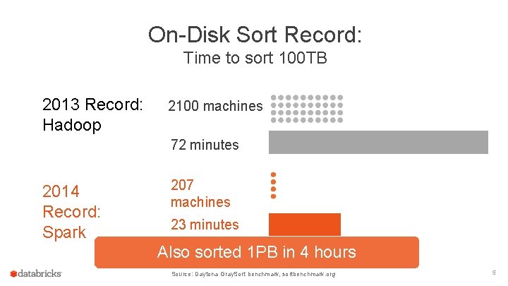
On-Disk Sort Record: Time to sort 100 TB 2013 Record: Hadoop 2100 machines 72 minutes 2014 Record: Spark 207 machines 23 minutes Also sorted 1 PB in 4 hours Source: Daytona Gray. Sort benchmark, sortbenchmark. org 5

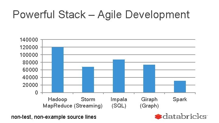
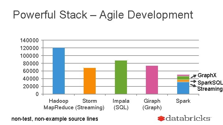
Powerful Stack – Agile Development 140000 120000 100000 80000 60000 40000 20000 0 Hadoop Storm Map. Reduce (Streaming) non-test, non-example source lines Impala (SQL) Giraph (Graph) Spark

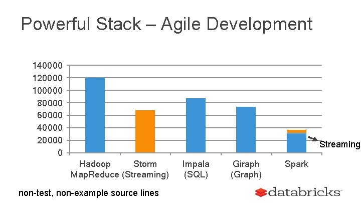
Powerful Stack – Agile Development 140000 120000 100000 80000 60000 40000 20000 0 Streaming Hadoop Storm Map. Reduce (Streaming) non-test, non-example source lines Impala (SQL) Giraph (Graph) Spark

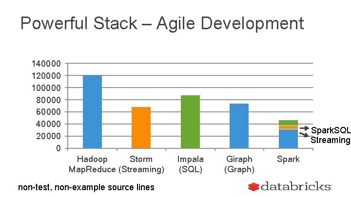
Powerful Stack – Agile Development 140000 120000 100000 80000 60000 40000 20000 0 Spark. SQL Streaming Hadoop Storm Map. Reduce (Streaming) non-test, non-example source lines Impala (SQL) Giraph (Graph) Spark

Powerful Stack – Agile Development 140000 120000 100000 80000 60000 40000 20000 0 Graph. X Spark. SQL Streaming Hadoop Storm Map. Reduce (Streaming) non-test, non-example source lines Impala (SQL) Giraph (Graph) Spark

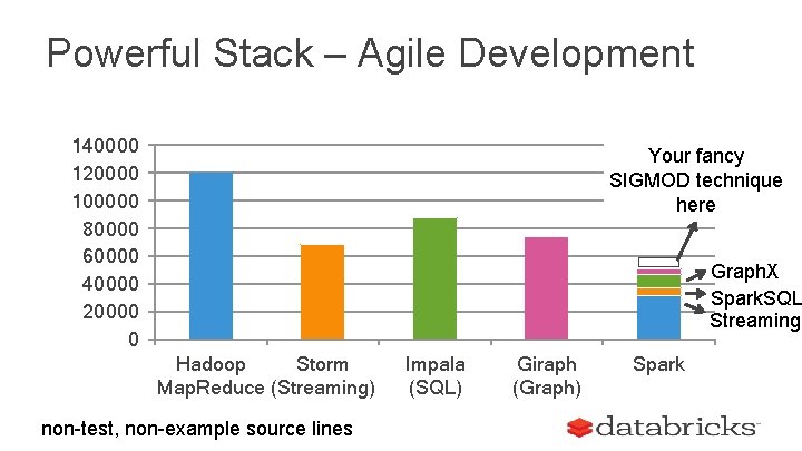
Powerful Stack – Agile Development 140000 120000 100000 80000 60000 40000 20000 0 Your fancy SIGMOD technique here Graph. X Spark. SQL Streaming Hadoop Storm Map. Reduce (Streaming) non-test, non-example source lines Impala (SQL) Giraph (Graph) Spark

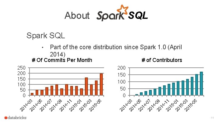
SQL About Spark SQL • Part of the core distribution since Spark 1. 0 (April 2014) # Of Commits Per Month 420 03 14 20 05 14 20 07 14 20 09 14 20 11 15 20 03 15 -0 5 20 1 503 20 1 501 20 1 411 20 1 409 20 1 407 20 1 405 200 150 100 50 0 403 250 200 150 100 50 0 # of Contributors 11

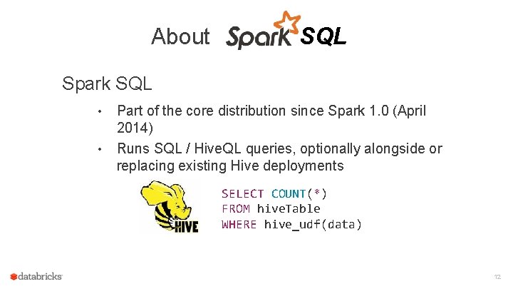
About SQL Spark SQL • • Part of the core distribution since Spark 1. 0 (April 2014) Runs SQL / Hive. QL queries, optionally alongside or replacing existing Hive deployments SELECT COUNT(*) FROM hive. Table WHERE hive_udf(data) 12

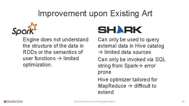
Improvement upon Existing Art Engine does not understand the structure of the data in RDDs or the semantics of user functions limited optimization. Can only be used to query external data in Hive catalog limited data sources Can only be invoked via SQL string from Spark error prone Hive optimizer tailored for Map. Reduce difficult to extend Set Footer from Insert Dropdown Menu 13

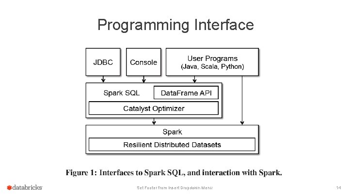
Programming Interface Set Footer from Insert Dropdown Menu 14

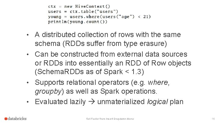
Data. Frame • A distributed collection of rows with the same schema (RDDs suffer from type erasure) • Can be constructed from external data sources or RDDs into essentially an RDD of Row objects (Schema. RDDs as of Spark < 1. 3) • Supports relational operators (e. g. where, groupby) as well as Spark operations. • Evaluated lazily unmaterialized logical plan Set Footer from Insert Dropdown Menu 15

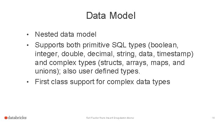
Data Model • Nested data model • Supports both primitive SQL types (boolean, integer, double, decimal, string, data, timestamp) and complex types (structs, arrays, maps, and unions); also user defined types. • First class support for complex data types Set Footer from Insert Dropdown Menu 16

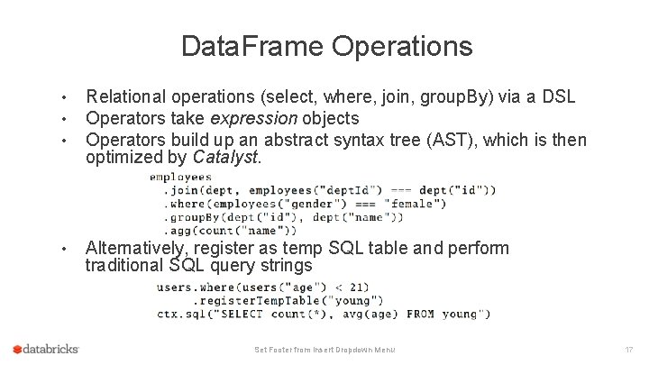
Data. Frame Operations • • • Relational operations (select, where, join, group. By) via a DSL Operators take expression objects Operators build up an abstract syntax tree (AST), which is then optimized by Catalyst. • Alternatively, register as temp SQL table and perform traditional SQL query strings Set Footer from Insert Dropdown Menu 17

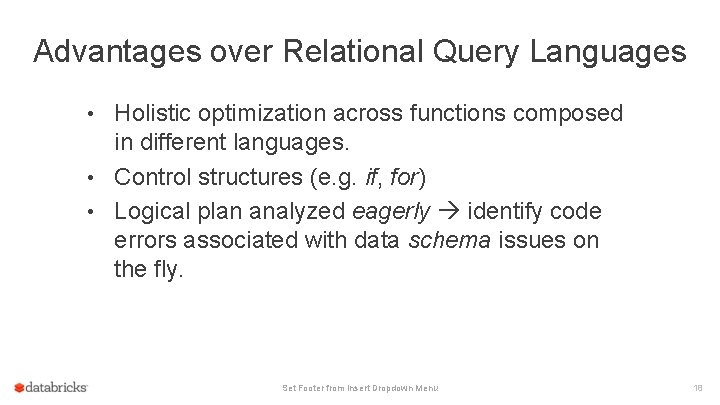
Advantages over Relational Query Languages • Holistic optimization across functions composed in different languages. • Control structures (e. g. if, for) • Logical plan analyzed eagerly identify code errors associated with data schema issues on the fly. Set Footer from Insert Dropdown Menu 18

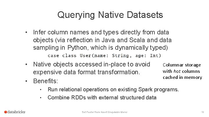
Querying Native Datasets • Infer column names and types directly from data objects (via reflection in Java and Scala and data sampling in Python, which is dynamically typed) • Native objects accessed in-place to avoid expensive data format transformation. • Benefits: • • Columnar storage with hot columns cached in memory Run relational operations on existing Spark programs. Combine RDDs with external structured data Set Footer from Insert Dropdown Menu 19

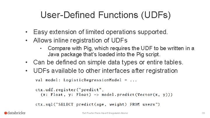
User-Defined Functions (UDFs) • Easy extension of limited operations supported. • Allows inline registration of UDFs • Compare with Pig, which requires the UDF to be written in a Java package that’s loaded into the Pig script. • Can be defined on simple data types or entire tables. • UDFs available to other interfaces after registration Set Footer from Insert Dropdown Menu 20

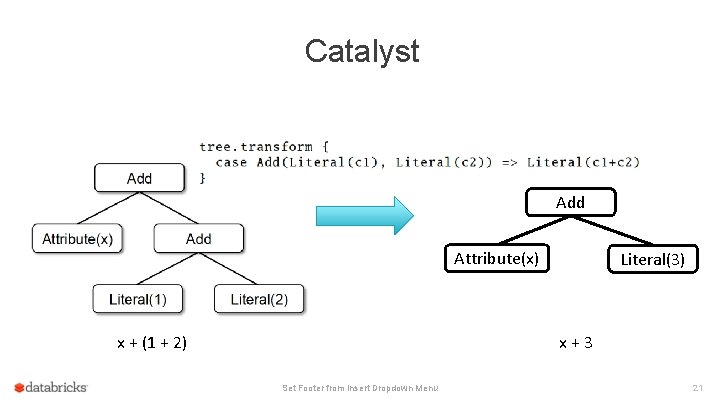
Catalyst Add Attribute(x) Literal(3) x+3 x + (1 + 2) Set Footer from Insert Dropdown Menu 21

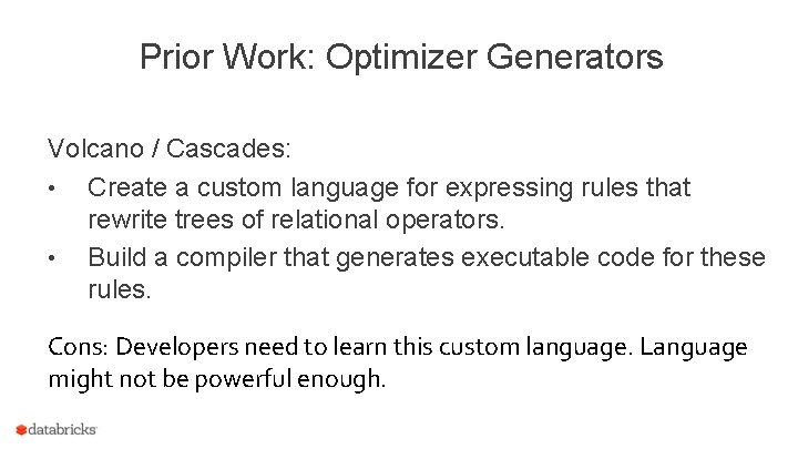
Prior Work: Optimizer Generators Volcano / Cascades: • Create a custom language for expressing rules that rewrite trees of relational operators. • Build a compiler that generates executable code for these rules. Cons: Developers need to learn this custom language. Language might not be powerful enough.

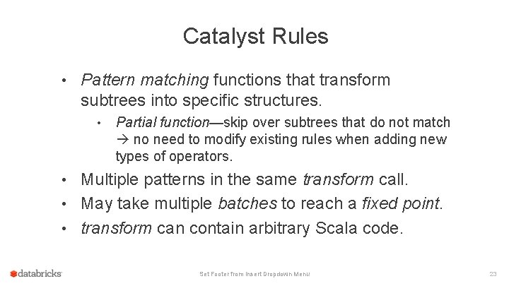
Catalyst Rules • Pattern matching functions that transform subtrees into specific structures. • Partial function—skip over subtrees that do not match no need to modify existing rules when adding new types of operators. • Multiple patterns in the same transform call. • May take multiple batches to reach a fixed point. • transform can contain arbitrary Scala code. Set Footer from Insert Dropdown Menu 23

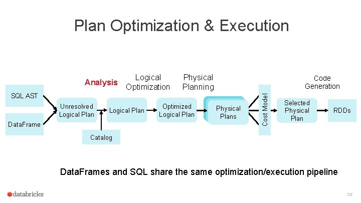
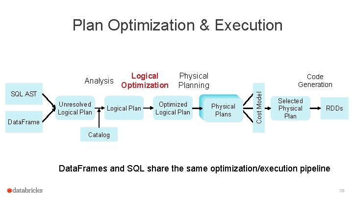
Plan Optimization & Execution Logical Optimization Physical Planning Code Generation SQL AST Unresolved Logical Plan Data. Frame Optimized Logical Plan Physical Plans Cost Model Analysis Selected Physical Plan RDDs Catalog Data. Frames and SQL share the same optimization/execution pipeline 24

Plan Optimization & Execution Logical Optimization Physical Planning Code Generation SQL AST Unresolved Logical Plan Data. Frame Optimized Logical Plan Physical Plans Cost Model Analysis Selected Physical Plan RDDs Catalog Data. Frames and SQL share the same optimization/execution pipeline 25

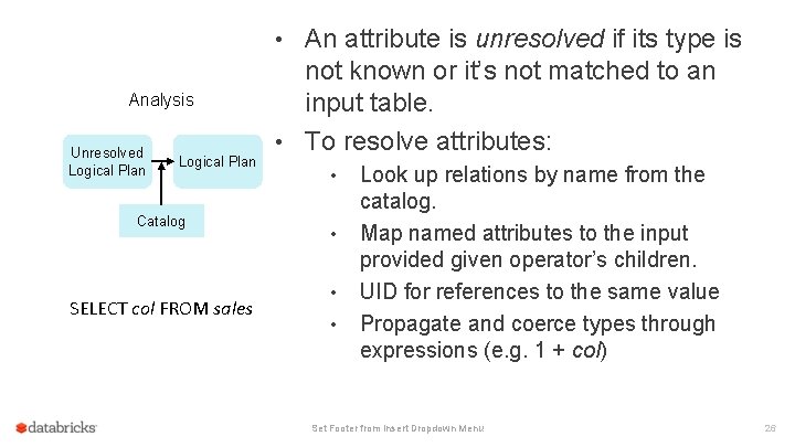
• An attribute is unresolved if its type is Analysis Unresolved Logical Plan Catalog SELECT col FROM sales not known or it’s not matched to an input table. • To resolve attributes: • • Look up relations by name from the catalog. Map named attributes to the input provided given operator’s children. UID for references to the same value Propagate and coerce types through expressions (e. g. 1 + col) Set Footer from Insert Dropdown Menu 26

Plan Optimization & Execution Logical Optimization Physical Planning Code Generation SQL AST Unresolved Logical Plan Data. Frame Optimized Logical Plan Physical Plans Cost Model Analysis Selected Physical Plan RDDs Catalog Data. Frames and SQL share the same optimization/execution pipeline 27

Plan Optimization & Execution Logical Optimization Physical Planning Code Generation SQL AST Unresolved Logical Plan Data. Frame Optimized Logical Plan Physical Plans Cost Model Analysis Selected Physical Plan RDDs Catalog Data. Frames and SQL share the same optimization/execution pipeline 28

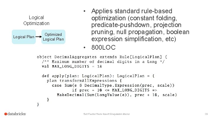
• Applies standard rule-based Logical Optimization Logical Plan Optimized Logical Plan optimization (constant folding, predicate-pushdown, projection pruning, null propagation, boolean expression simplification, etc) • 800 LOC Set Footer from Insert Dropdown Menu 29

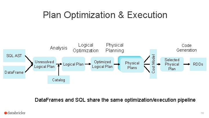
Plan Optimization & Execution Logical Optimization Physical Planning Code Generation SQL AST Unresolved Logical Plan Data. Frame Optimized Logical Plan Physical Plans Cost Model Analysis Selected Physical Plan RDDs Catalog Data. Frames and SQL share the same optimization/execution pipeline 30

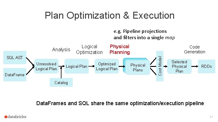
Plan Optimization & Execution e. g. Pipeline projections and filters into a single map Logical Optimization Physical Planning Code Generation SQL AST Unresolved Logical Plan Data. Frame Optimized Logical Plan Physical Plans Cost Model Analysis Selected Physical Plan RDDs Catalog Data. Frames and SQL share the same optimization/execution pipeline 31

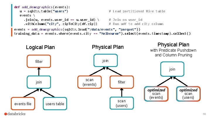
def add_demographics(events): u = sql. Ctx. table("users") events . join(u, events. user_id == u. user_id) . with. Column("city", zip. To. City(df. zip)) # Load partitioned Hive table # Join on user_id # Run udf to add city column events = add_demographics(sql. Ctx. load("/data/events", "parquet")) training_data = events. where(events. city == "Melbourne"). select(events. timestamp). collect() Logical Plan Physical Plan with Predicate Pushdown and Column Pruning join filter join scan (events) join events file users table filter scan (users) optimized scan (events) optimized scan (users) 32

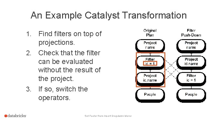
An Example Catalyst Transformation Find filters on top of projections. 2. Check that the filter can be evaluated without the result of the project. 3. If so, switch the operators. 1. Set Footer from Insert Dropdown Menu

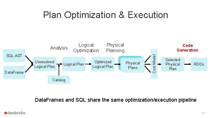
Plan Optimization & Execution Logical Optimization Physical Planning Code Generation SQL AST Unresolved Logical Plan Data. Frame Optimized Logical Plan Physical Plans Cost Model Analysis Selected Physical Plan RDDs Catalog Data. Frames and SQL share the same optimization/execution pipeline 34

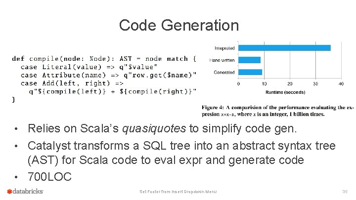
Code Generation • Relies on Scala’s quasiquotes to simplify code gen. • Catalyst transforms a SQL tree into an abstract syntax tree (AST) for Scala code to eval expr and generate code • 700 LOC Set Footer from Insert Dropdown Menu 35

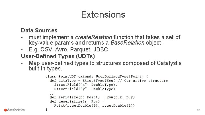
Extensions Data Sources • must implement a create. Relation function that takes a set of key-value params and returns a Base. Relation object. • E. g. CSV, Avro, Parquet, JDBC User-Defined Types (UDTs) • Map user-defined types to structures composed of Catalyst’s built-in types. Set Footer from Insert Dropdown Menu 36

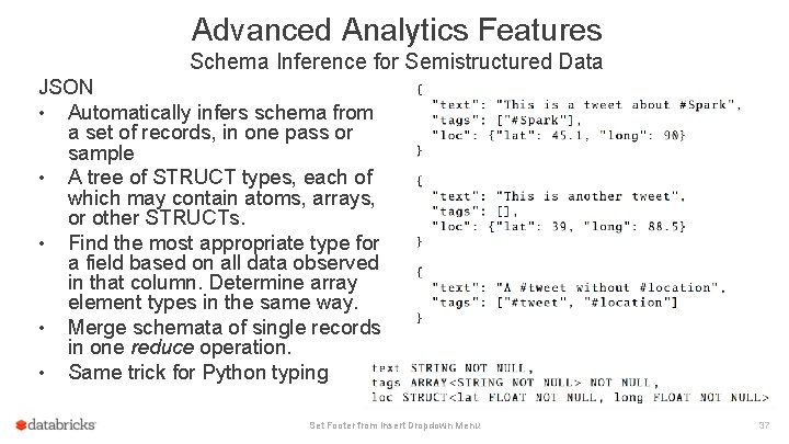
Advanced Analytics Features Schema Inference for Semistructured Data JSON • Automatically infers schema from a set of records, in one pass or sample • A tree of STRUCT types, each of which may contain atoms, arrays, or other STRUCTs. • Find the most appropriate type for a field based on all data observed in that column. Determine array element types in the same way. • Merge schemata of single records in one reduce operation. • Same trick for Python typing Set Footer from Insert Dropdown Menu 37

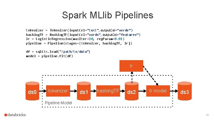
Spark MLlib Pipelines tokenizer = Tokenizer(input. Col="text", output. Col="words”) hashing. TF = Hashing. TF(input. Col="words", output. Col="features”) lr = Logistic. Regression(max. Iter=10, reg. Param=0. 01) pipeline = Pipeline(stages=[tokenizer, hashing. TF, lr]) df = sql. Ctx. load("/path/to/data") model = pipeline. fit(df) lr ds 0 tokenizer ds 1 hashing. TF ds 2 lr. model ds 3 Pipeline Model 38

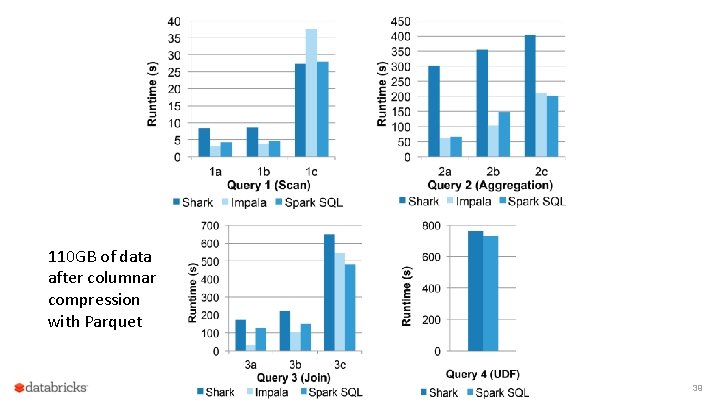
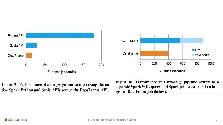
110 GB of data after columnar compression with Parquet Set Footer from Insert Dropdown Menu 39

Set Footer from Insert Dropdown Menu 40

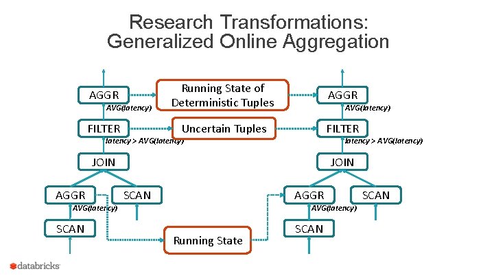
Research Transformations: Generalized Online Aggregation AGGR AVG(latency) FILTER Running State of Deterministic Tuples AGGR Uncertain Tuples FILTER AVG(latency) latency > AVG(latency) JOIN AGGR JOIN SCAN AGGR AVG(latency) SCAN AVG(latency) Running State SCAN

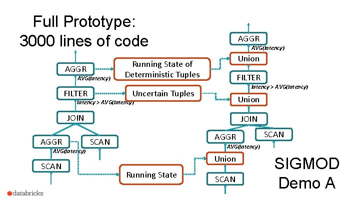
Full Prototype: 3000 lines of code AGGR AVG(latency) Union Running State of Deterministic Tuples FILTER latency > AVG(latency) Uncertain Tuples FILTER Union latency > AVG(latency) JOIN AGGR SCAN AVG(latency) SCAN Union Running State SCAN SIGMOD Demo A

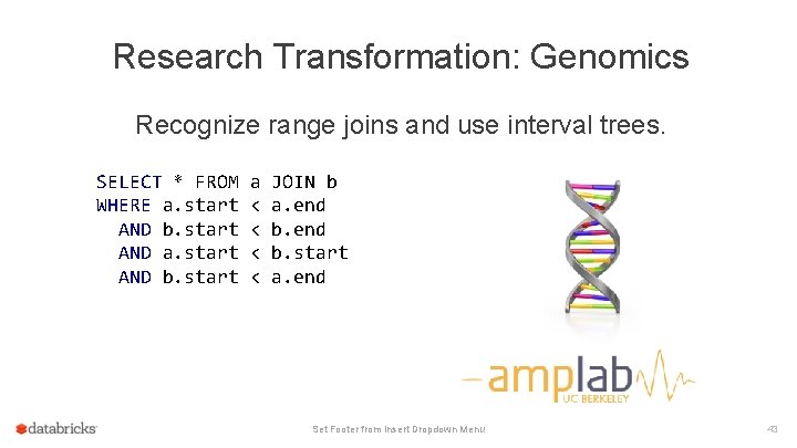
Research Transformation: Genomics Recognize range joins and use interval trees. SELECT * FROM WHERE a. start AND b. start AND a. start AND b. start a < < JOIN b a. end b. start a. end Set Footer from Insert Dropdown Menu 43

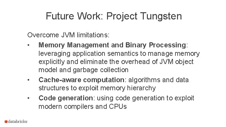
Future Work: Project Tungsten Overcome JVM limitations: • Memory Management and Binary Processing: leveraging application semantics to manage memory explicitly and eliminate the overhead of JVM object model and garbage collection • Cache-aware computation: algorithms and data structures to exploit memory hierarchy • Code generation: using code generation to exploit modern compilers and CPUs

Questions?

The not-so-secret truth. . . SQL is about more than SQL. 48

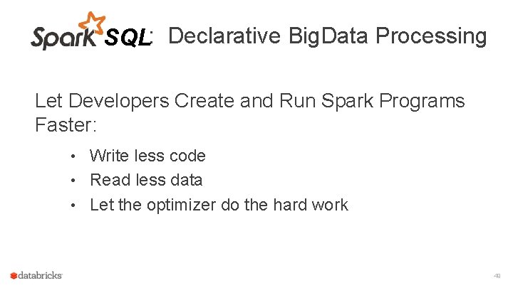
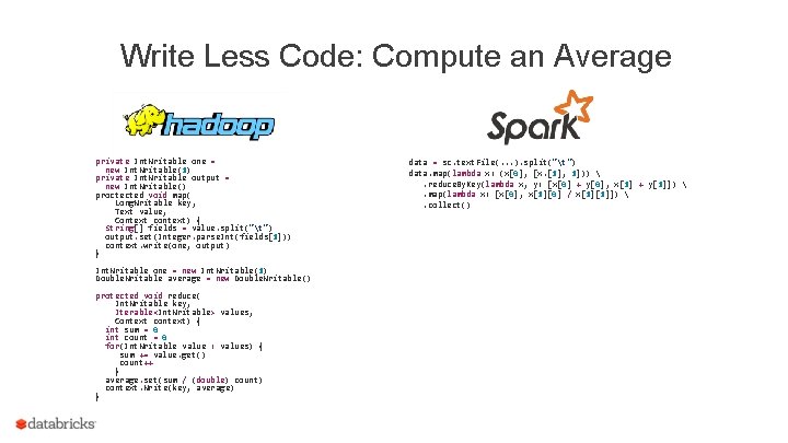
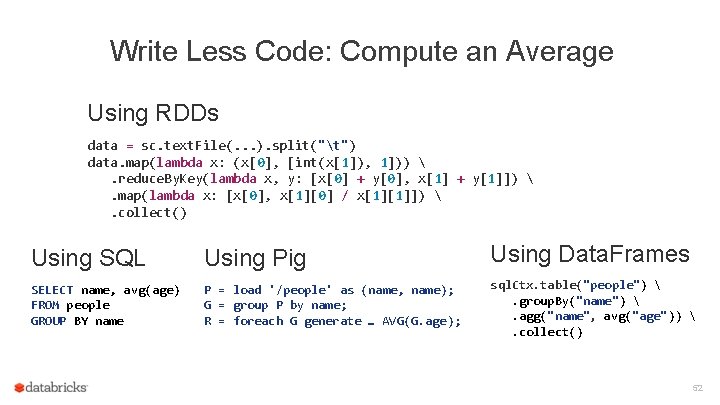
SQL: Declarative Big. Data Processing Let Developers Create and Run Spark Programs Faster: • Write less code • Read less data • Let the optimizer do the hard work 49

Data. Frame noun – [dey-tuh-freym] 1. A distributed collection of rows organized into named columns. 2. An abstraction for selecting, filtering, aggregating and plotting structured data (cf. R, Pandas). 3. Archaic: Previously Schema. RDD (cf. Spark < 1. 3). 50

Write Less Code: Compute an Average private Int. Writable one = new Int. Writable(1) private Int. Writable output = new Int. Writable() proctected void map( Long. Writable key, Text value, Context context) { String[] fields = value. split("t") output. set(Integer. parse. Int(fields[1])) context. write(one, output) } Int. Writable one = new Int. Writable(1) Double. Writable average = new Double. Writable() protected void reduce( Int. Writable key, Iterable<Int. Writable> values, Context context) { int sum = 0 int count = 0 for(Int. Writable value : values) { sum += value. get() count++ } average. set(sum / (double) count) context. Write(key, average) } data = sc. text. File(. . . ). split("t") data. map(lambda x: (x[0], [x. [1], 1])) . reduce. By. Key(lambda x, y: [x[0] + y[0], x[1] + y[1]]) . map(lambda x: [x[0], x[1][0] / x[1][1]]) . collect()

Write Less Code: Compute an Average Using RDDs data = sc. text. File(. . . ). split("t") data. map(lambda x: (x[0], [int(x[1]), 1])) . reduce. By. Key(lambda x, y: [x[0] + y[0], x[1] + y[1]]) . map(lambda x: [x[0], x[1][0] / x[1][1]]) . collect() Using SQL Using Pig Using Data. Frames SELECT name, avg(age) FROM people GROUP BY name P = load '/people' as (name, name); G = group P by name; R = foreach G generate … AVG(G. age); sql. Ctx. table("people") . group. By("name") . agg("name", avg("age")) . collect() 52

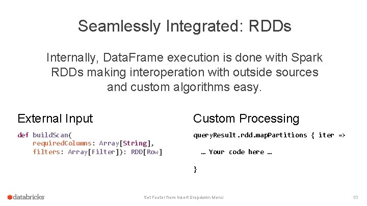
Seamlessly Integrated: RDDs Internally, Data. Frame execution is done with Spark RDDs making interoperation with outside sources and custom algorithms easy. External Input Custom Processing def build. Scan( required. Columns: Array[String], filters: Array[Filter]): RDD[Row] query. Result. rdd. map. Partitions { iter => … Your code here … } Set Footer from Insert Dropdown Menu 53

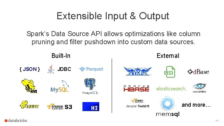
Extensible Input & Output Spark’s Data Source API allows optimizations like column pruning and filter pushdown into custom data sources. Built-In { JSON } External JDBC and more… 54

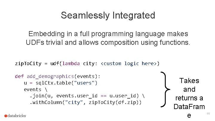
Seamlessly Integrated Embedding in a full programming language makes UDFs trivial and allows composition using functions. zip. To. City = udf(lambda city: <custom logic here>) def add_demographics(events): u = sql. Ctx. table("users") events . join(u, events. user_id == u. user_id) . with. Column("city", zip. To. City(df. zip)) Takes and returns a Data. Fram e 55

Spark MLlib Pipelines tokenizer = Tokenizer(input. Col="text", output. Col="words”) hashing. TF = Hashing. TF(input. Col="words", output. Col="features”) lr = Logistic. Regression(max. Iter=10, reg. Param=0. 01) pipeline = Pipeline(stages=[tokenizer, hashing. TF, lr]) df = sql. Ctx. load("/path/to/data") model = pipeline. fit(df) lr ds 0 tokenizer ds 1 hashing. TF ds 2 lr. model ds 3 Pipeline Model 56