Spanning Tree A spanning tree is any tree

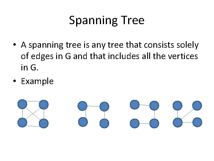
Spanning Tree • A spanning tree is any tree that consists solely of edges in G and that includes all the vertices in G. • Example

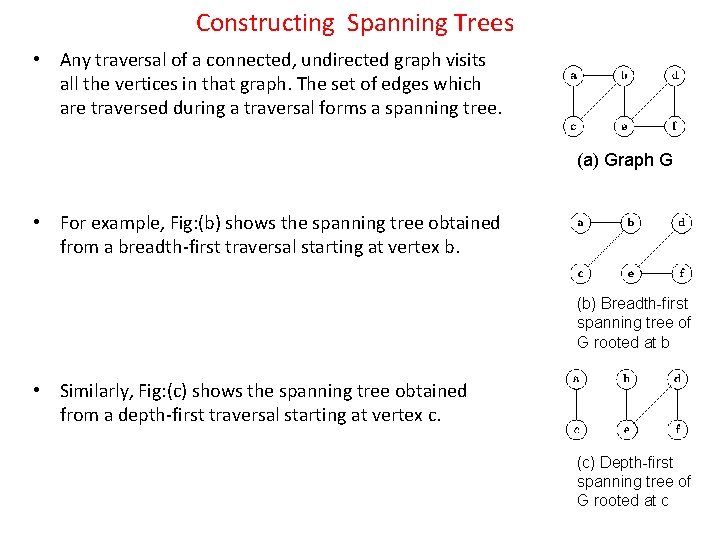
Constructing Spanning Trees • Any traversal of a connected, undirected graph visits all the vertices in that graph. The set of edges which are traversed during a traversal forms a spanning tree. (a) Graph G • For example, Fig: (b) shows the spanning tree obtained from a breadth-first traversal starting at vertex b. (b) Breadth-first spanning tree of G rooted at b • Similarly, Fig: (c) shows the spanning tree obtained from a depth-first traversal starting at vertex c. (c) Depth-first spanning tree of G rooted at c

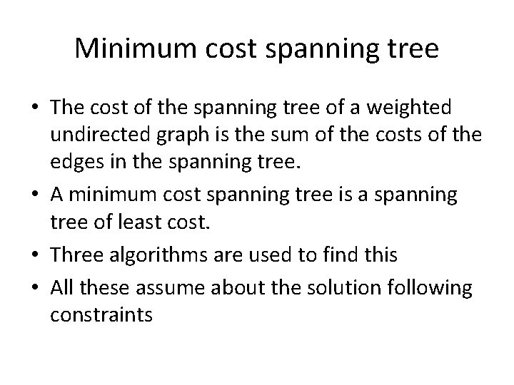
Minimum cost spanning tree • The cost of the spanning tree of a weighted undirected graph is the sum of the costs of the edges in the spanning tree. • A minimum cost spanning tree is a spanning tree of least cost. • Three algorithms are used to find this • All these assume about the solution following constraints

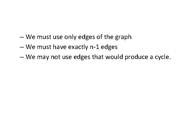
– We must use only edges of the graph – We must have exactly n-1 edges – We may not use edges that would produce a cycle.

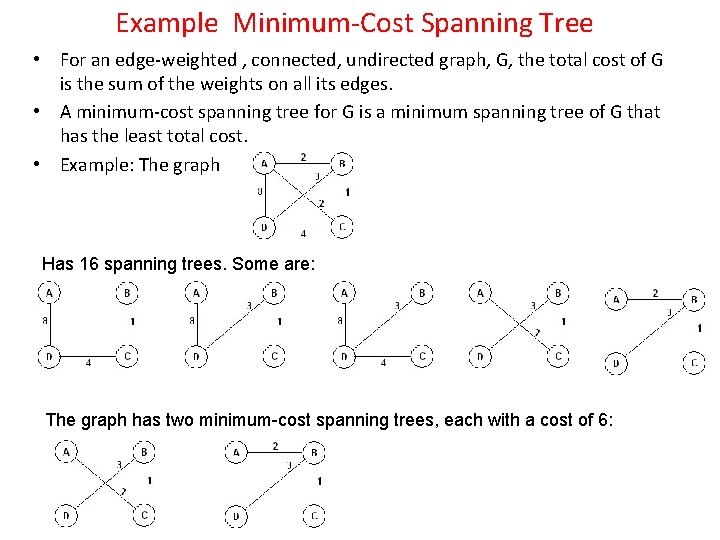
Example Minimum-Cost Spanning Tree • For an edge-weighted , connected, undirected graph, G, the total cost of G is the sum of the weights on all its edges. • A minimum-cost spanning tree for G is a minimum spanning tree of G that has the least total cost. • Example: The graph Has 16 spanning trees. Some are: The graph has two minimum-cost spanning trees, each with a cost of 6:

Applications of Minimum-Cost Spanning Trees Minimum-cost spanning trees have many applications. Some are: • Building cable networks that join n locations with minimum cost. • Building a road network that joins n cities with minimum cost. • Obtaining an independent set of circuit equations for an electrical network. • In pattern recognition minimal spanning trees can be used to find noisy pixels.

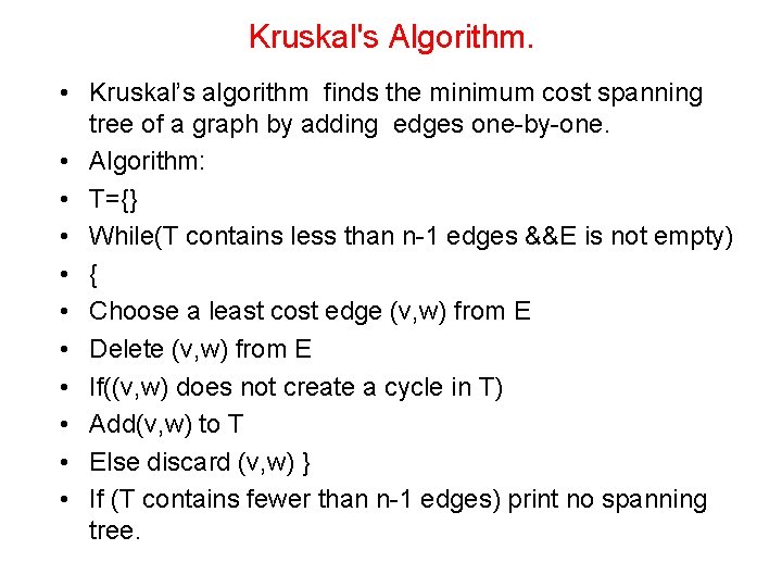
Kruskal's Algorithm. • Kruskal’s algorithm finds the minimum cost spanning tree of a graph by adding edges one-by-one. • Algorithm: • T={} • While(T contains less than n-1 edges &&E is not empty) • { • Choose a least cost edge (v, w) from E • Delete (v, w) from E • If((v, w) does not create a cycle in T) • Add(v, w) to T • Else discard (v, w) } • If (T contains fewer than n-1 edges) print no spanning tree.

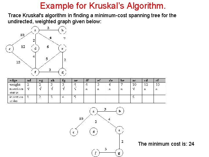
Example for Kruskal’s Algorithm. Trace Kruskal's algorithm in finding a minimum-cost spanning tree for the undirected, weighted graph given below: The minimum cost is: 24

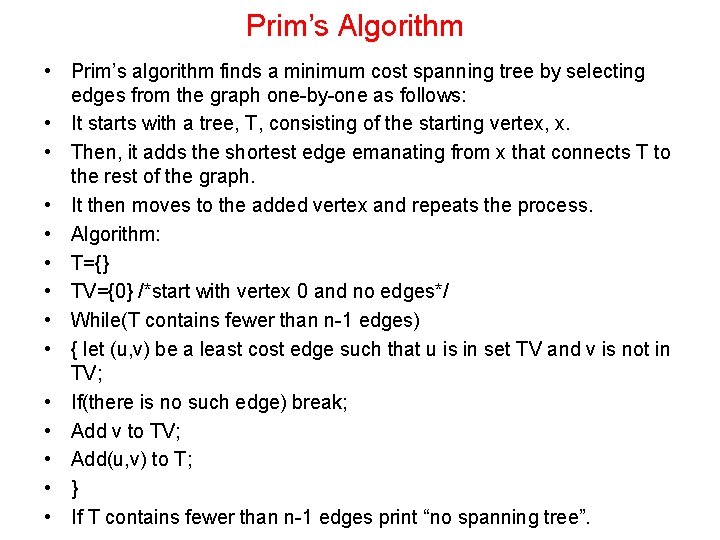
Prim’s Algorithm • Prim’s algorithm finds a minimum cost spanning tree by selecting edges from the graph one-by-one as follows: • It starts with a tree, T, consisting of the starting vertex, x. • Then, it adds the shortest edge emanating from x that connects T to the rest of the graph. • It then moves to the added vertex and repeats the process. • Algorithm: • T={} • TV={0} /*start with vertex 0 and no edges*/ • While(T contains fewer than n-1 edges) • { let (u, v) be a least cost edge such that u is in set TV and v is not in TV; • If(there is no such edge) break; • Add v to TV; • Add(u, v) to T; • } • If T contains fewer than n-1 edges print “no spanning tree”.

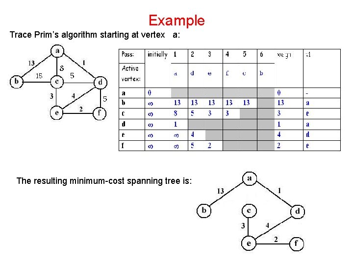
Example Trace Prim’s algorithm starting at vertex a: The resulting minimum-cost spanning tree is:

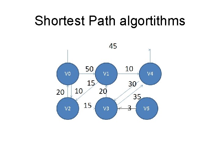
Shortest Path algortithms

Dijikstra’s Algorithm • • #define MAX_VERTICES 6 int cost[][MAX_VERTICES]={ {0, 50, 1000, 45, 1000}, {1000, 0, 15, 1000, 1000}, {20, 1000, 0, 15, 1000}, {1000, 20, 1000, 0, 35, 1000}, {1000, 30, 1000, 0, 1000}, {1000, 3, 1000, 0}};

• • • int dist[MAX_VERTICES]; short int found[MAX_VERTICES]={0}; int n=MAX_VERTICES; int choose(int dist[], int n, short int found[]) { int i, minpos; min=32767; minpos=-1; for(i=0; i<n; i++){ If(dist[i]<min && !found[i]){ min=dist[i]; minpos=i; } return minpos; }

• void shortestpath(int v, int cost[][MAX_VERTICES], int dist[], int n, short int found){ • /*dist[i] represents shortest path from vertex v to i. found[i] holds 0 if shortest path to vertex i has not been found 1 otherwise. */ • int i, u, w; • for(i=0; i<n; i++){ dist[i]=cost[v][i]; } • found[v]=1; dist[v]=0;

• • for(i=0; i<n-2; i++){ u=choose(dist, n, found); found[u]=1; for(w=0; w<n; w++) if(!found[w]) if(dist[u]+cost[u][w]<dist[w]) dist[w]=dist[u]+cost[u][w]; } }

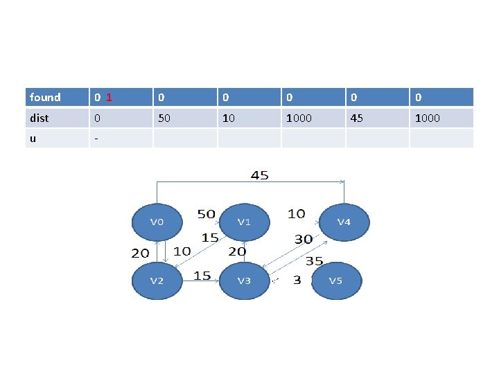
found 0 0 0 dist 0 50 10 1000 45 1000 u -

found 0 1 0 0 0 dist 0 50 10 1000 45 1000 u -

found 01 0 0 0 dist 0 50 10 1000 25 45 1000 u 2

found 0 1 0 1 0 0 dist 0 50 45 10 1000 25 45 1000 u 3

found 0 1 0 1 0 0 dist 0 50 45 10 1000 25 45 1000 u 1

found 0 1 0 1 0 1 0 dist 0 50 45 10 1000 25 45 1000 u 4

All pairs Shortest Path algorithm • void allcosts(int cost[][MAX_VERTICES], int dist[][MAX_VERTICES], int n){ • /* determine the distances from each vertex to every other vertex, cost is the adjacency matrix , dist is the matrix of distances*/ • int i, j, k; • for(i=0; i<n; i++) • for(j=0; j<n; j++) • {dist[i][j]=cost[i][j]; }

• • • for(k=0; k<n; k++) for(i=0; i<n; i++) for(j=0; j<n; j++) if(dist[i][k]+dist[k][j]<dist[i][j]) Dist[i][j]=dist[i][k]+dist[k][j]; }

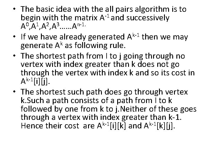
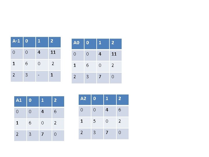
• The basic idea with the all pairs algorithm is to begin with the matrix A-1 and successively A 0, A 1, A 2, A 3……An-1. • If we have already generated Ak-1 then we may generate Ak as following rule. • The shortest path from I to j going through no vertex with index greater than k does not go through the vertex with index k and so its cost in Ak-1[i][j]. • The shortest such path does go through vertex k. Such a path consists of a path from I to k followed by one from k to j. Neither of these goes through a vertex with index greater than k-1. Hence their cost are Ak-1[i][k] and Ak-1[k][j].

• Ak[i][j]=min{Ak-1[i][j], Ak-1[i][k]+Ak-1[k][j]}, k>=0 • A-1[i][j]=cost[i][j].

A-1 0 1 2 A 0 0 1 2 0 0 4 11 1 6 0 2 2 3 - 1 2 3 7 0 A 1 0 1 2 A 2 0 1 2 0 0 4 6 1 6 0 2 1 5 0 2 2 3 7 0

Transitive closure