Source localization for EEG and MEG Methods for

Source localization for EEG and MEG Methods for Dummies 2006 FIL Bahador Bahrami

Before we start … • SPM 5 and source localization: • On-going work in progress • MFD and source localization: • This is the first on this topic • Main references for this talk: • Jeremie Mattout’s slides from SPM course • Slotnick S. D. chapter in Todd Handy’s ERP handbook • Rimona Weil’s wonderful help (thanks Rimona!)

Outline • Theoretical • Source localization stated as a problem • Solution to the problem and their limitations • Practical* • • How to prepare data Which buttons to press What to avoid What to expect * Subject to change along with the development of SPM 5

Source localization as a problem

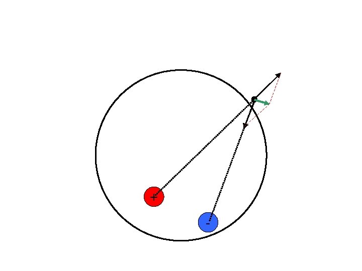
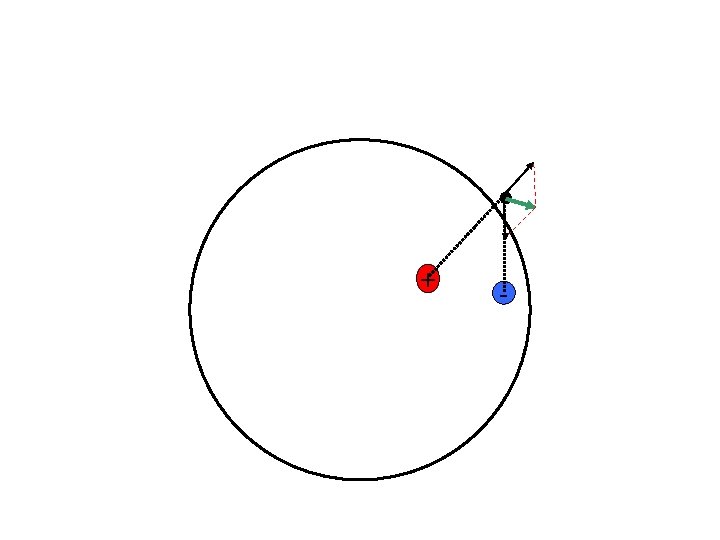
+ + - Any field potential vector could be consistent with an infinite number of possible dipoles The possibilities only increase with tri-poles and quadra-poles -

ERP and MEG give us

And source localization aims to infer + among

How do we know which one is correct? + + - We can’t. There is no correct answer. Source localization is an ILL-DEFINED PROBLEM We can only see which one is better Can we find the best answer? Only among the alternatives that you have considered. -

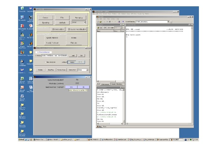
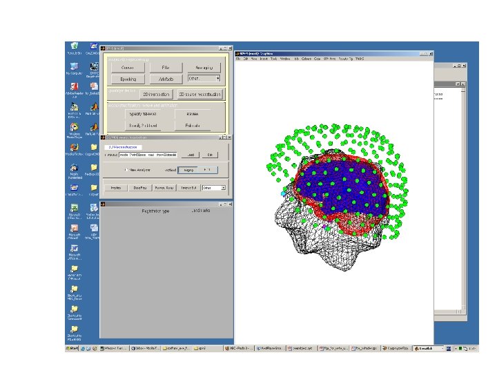
HUNTING for best possible solution Step ONE: How does your data look like? MEG sensor location Source Reconstruction Registration MEG data

HUNTING for best possible solution Step Two If then If If FORWARD MODEL then And on and …

HUNTING for best possible solution Forward Model Experimental DATA Inverse Solution Which forward solutions fit the DATA better (less error)?

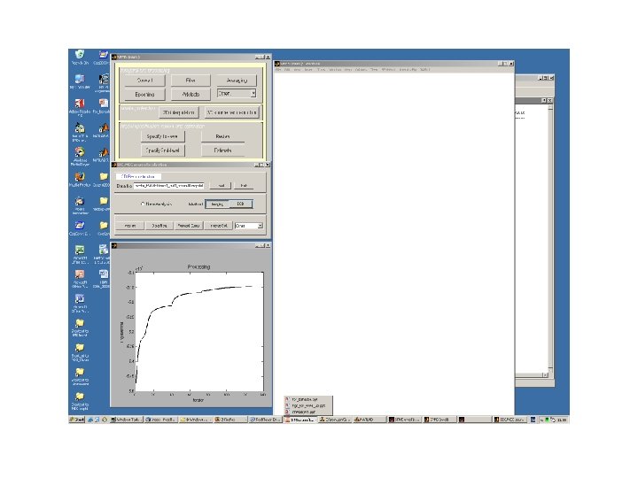
HUNTING for best possible solution Forward DATA Iterative Process Until solution stops getting better (error stabilises) error Inverse Solution iteration

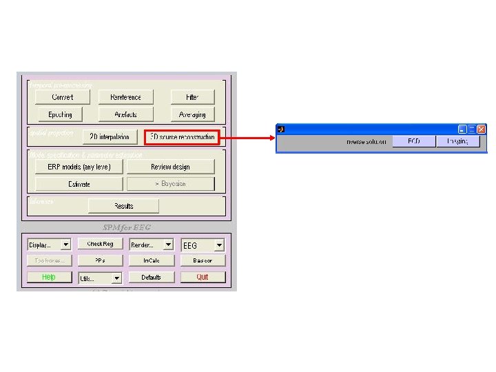
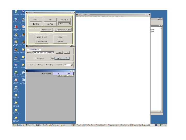
Components of the source reconstruction process Source model ‘ECD’ ‘Imaging’ Forward model Registration Inverse method Data Anatomy

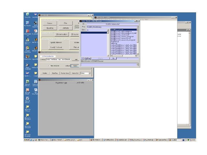
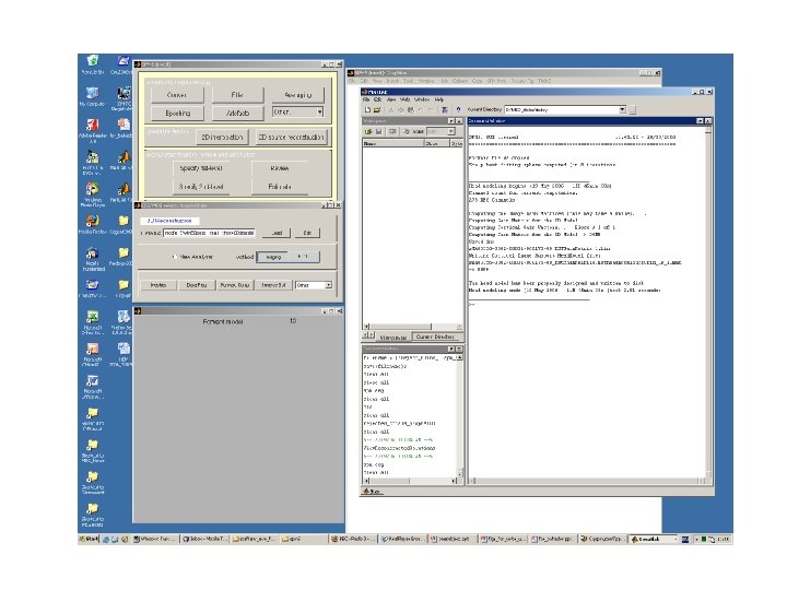
Recipe for Source localization in SPM 5 • Ingredients – MEG converter has given you All in the same folder • • . MAT data file (contains experimental data) sensloc file (sensors locations) sensorient (sensors orientations) fidloc (fiducial locations in MEG space) – fidloc in MRI space (we will see shortly) – Structural T 1 MRI scan

fidloc in MRI space X Nasion YNasion Z Nasion X Left Tragus YLeft Tragus Z Left Tragus X Right Tragus YRight Tragus Z Right Tragus Get these using SPM Display button Save it as a MAT file in the same directory as the data

Components of the source reconstruction process Source model Registration Forward model Inverse solution

Source model

Source model Compute transformation T Individual MRI Templates Apply inverse transformation T-1 Individual mesh functions - Individual MRI - Template mesh - spatial normalization into MNI template - inverted transformation applied to the template mesh output - individual mesh

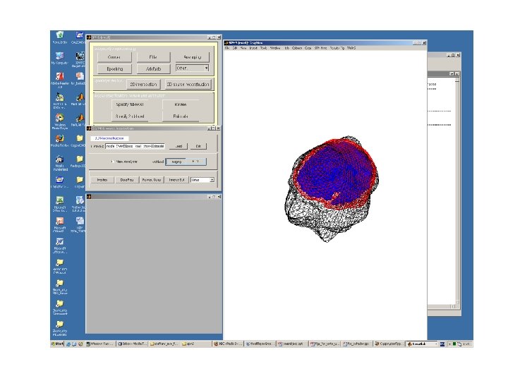
Scalp Mesh iskull mesh

Components of the source reconstruction process Registration

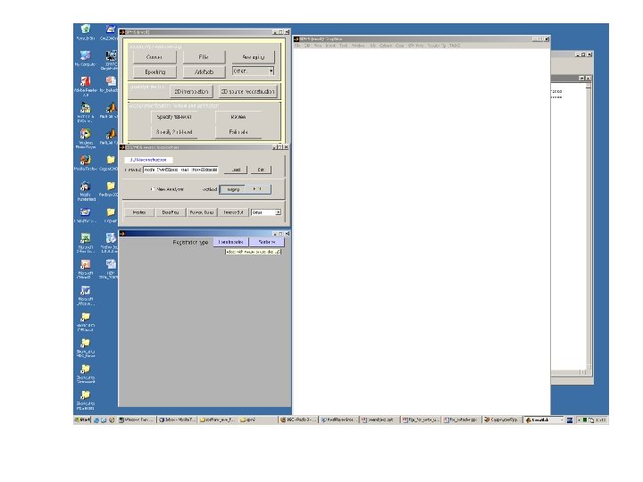
Registration fiducials Rigid transformation (R, t) Individual sensor space Individual MRI space input - sensor locations - fiducial locations (in both sensor & MRI space) - individual MRI functions - registration of the EEG/MEG data into individual MRI space output - registrated data - rigid transformation

Forward model

Foward model Compute for each dipole + K n Forward operator Individual MRI space input - sensor locations - individual mesh Model of the head tissue properties functions - single sphere - three spheres - overlapping spheres - realistic spheres Brain. Storm output - forward operator K

Inverse solution

Inverse solution (1) - General principles General Linear Model 1 dipole source per location Cortical mesh Under-determined GLM Regularized solution Y = KJ+ E [nxt] [nxp][pxt] [nxt] n : number of sensors p : number of dipoles t : number of time samples ||Y – KJ||2 + λf(J) ) J^ : min( J data fit priors

Inverse solution (2) - Parametric empirical Bayes 2 -level hierarchical model Gaussian variables with unknown variance Y = KJ + E 1 ~ N(0, Ce) J = 0 + E 2 Sensor level E 2 ~ N(0, Cp) Source level Linear parametrization of the variances Ce = 1. Qe 1 + … + q. Qeq Cp = λ 1. Qp 1 + … + λk. Qpk Q: variance components ( , λ): hyperparameters

Inverse solution (3) - Parametric empirical Bayesian inference on model parameters + Model M + J Q e 1 , … , Q eq Q p 1 , … , Q pk , λ K Inference on J and ( , λ) Maximizing the log-evidence F = log( p(Y|M) ) = log( p(Y|J, M) ) + log( p(J|M) ) d. J data fit priors Expectation-Maximization (EM) E-step: maximizing F wrt J M-step: maximizing of F wrt ( , λ) J^ = CJKT[Ce + KCJ KT]-1 Y MAP estimate Ce + KCJKT = E[YYT] Re. ML estimate

Inverse solution (4) - Parametric empirical Bayesian model comparison Model evidence • Relevance of model M is quantified by its evidence p(Y|M) maximized by the EM scheme Model comparison • Two models M 1 and M 2 can be compared by the ratio of their evidence B 12 = p(Y|M 1) p(Y|M 2) Bayes factor Model selection using a ‘Leaving-one-prior-out-strategy‘

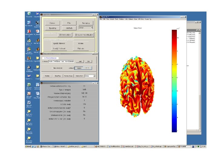
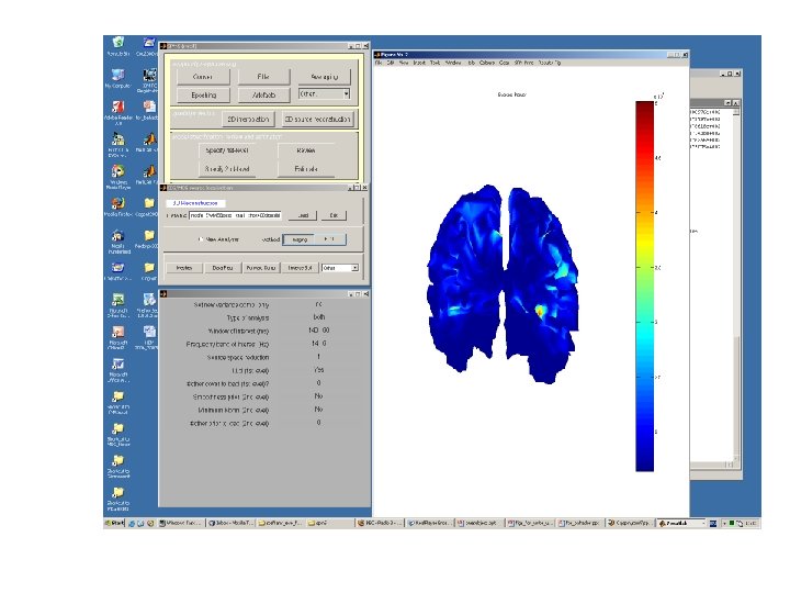
Inverse solution (5) - implementation input - preprocessed data - forward operator - individual mesh - priors functions - compute the MAP estimate of J - compute the Re. ML estimate of ( , λ) - interpolate into individual MRI voxel-space ECD approach - iterative forward and inverse computation output - inverse estimate - model evidence

HUNTING for best possible solution Forward DATA Iterative Process Until solution stops getting better (error stabilises) error Inverse Solution iteration

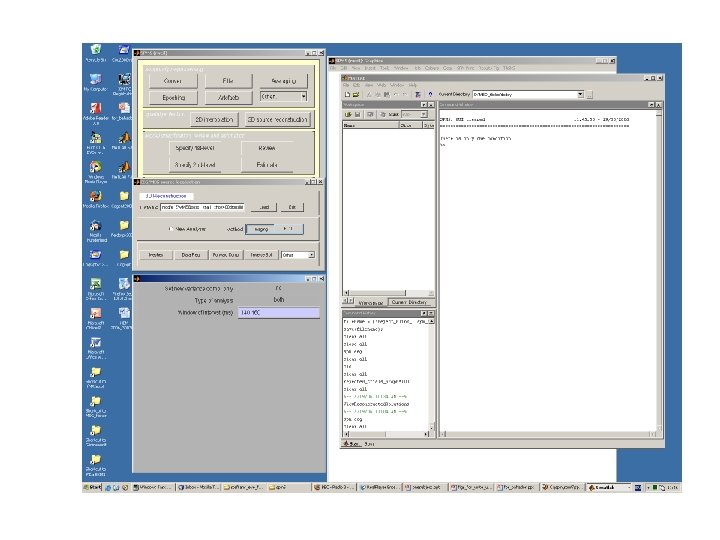
Types of Analysis Jeremie says: • Evoked – The evoked response is a reproducible response which occurs after each stimulation and is phase-locked with the stimulus onset. • Induced – The induced response is usually characterized in the frequency domain and contrary to the evoked response, is not phased-locked with the stimulus onset. • • The evoked response is obtained (on the scalp) as the stimulus or eventlocked average over trials. This is then the input data for the 'evoked' case in source reconstruction. One can also reconstruct the evoked power in some frequency band (over the time window), this is what is obtained when choosing 'both' in source reconstruction.

Conclusion - Summary MRI space Data space Registration Forward model EEG/MEG preprocessed data PEB inverse solution SPM

Important! Source model The same for all conditions. Therefore, only done ONCE for each subject Registra tion Forward model Inverse solution Repeated for each condition

Considerations • Source localization project is still ongoing • Unable to incorporate prior assumptions about source (e. g. , from f. MRI blobs) • Source localization only for conditions • Not for contrasts • Source localization is a single subject analysis (no way to look at group effects)

Thank you Rimona! Thank you MFD!