Sorting CSIT 402 Data Structures II Sorting Ascending

Sorting CSIT 402 Data Structures II

Sorting (Ascending Order) • Input › an array A of data records › a key value in each data record › a comparison function which imposes a consistent ordering on the keys (e. g. , integers) • Output › reorganize the elements of A such that • For any i and j, if i < j then A[i] A[j] 2

Space • How much space does the sorting algorithm require in order to sort the collection of items? › › Is copying needed? O(n) time to accomplish In-place sorting – no copying – O(1) time Somewhere in between for “temporary”, space External memory sorting – data so large that does not fit in memory 3

Time • How fast is the algorithm? › The definition of a sorted array A says that for any i<j, A[i] < A[j] › This means that you need to at least check on each element at the very minimum, I. e. , at least O(N) › And you could end up checking each element against every other element, which is O(N 2) › The big question is: How close to O(N) can you get? 4

Stability • Stability: Does it rearrange the order of input data records which have the same key value (duplicates)? › E. g. Phone book sorted by name. Now sort by county – is the list still sorted by name within each county? › Extremely important property for databases › A stable sorting algorithm is one which does not rearrange the order of duplicate keys 5

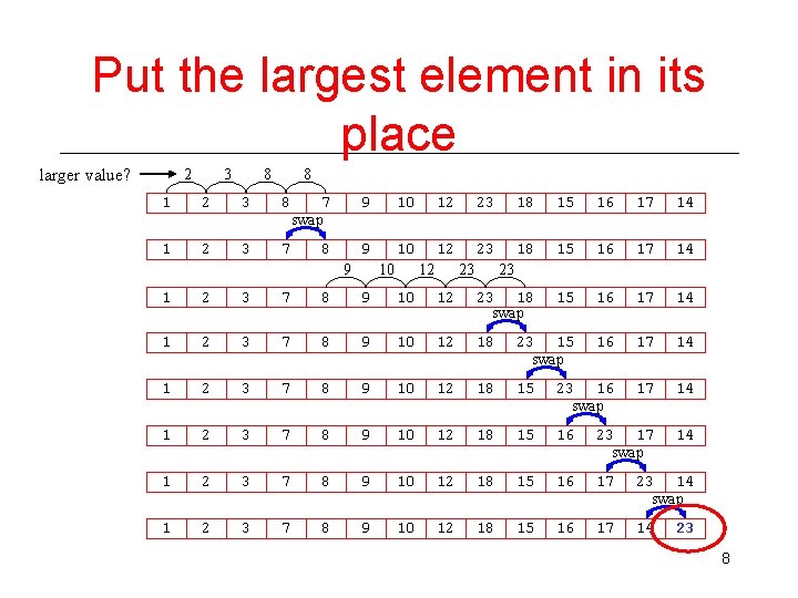
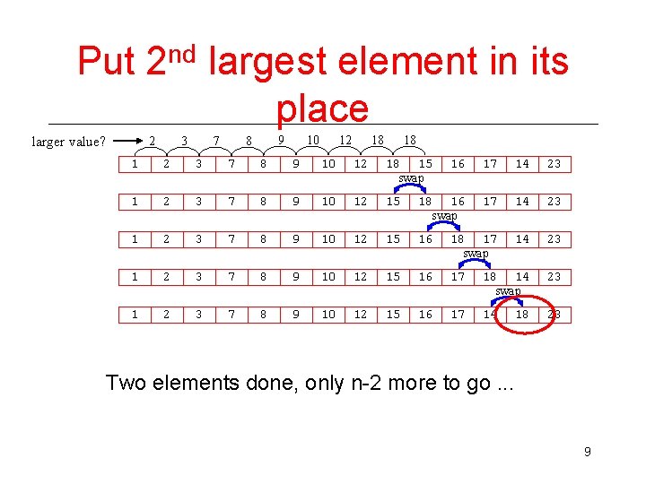
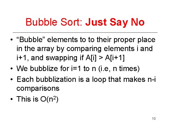
Bubble Sort • “Bubble” elements to to their proper place in the array by comparing elements i and i+1, and swapping if A[i] > A[i+1] › Bubble every element towards its correct position • last position has the largest element • then bubble every element except the last one towards its correct position • then repeat until done or until the end of the quarter, whichever comes first. . . 6

Bubblesort bubble(A[1. . n]: integer array, n : integer): { i, j : integer; for i = 1 to n-1 do for j = 2 to n–i+1 do if A[j-1] > A[j] then SWAP(A[j-1], A[j]); } SWAP(a, b) : { t : integer; 6 t: =a; a: =b; b: =t; } 1 2 3 4 5 6 6 5 3 2 7 1 5 6 3 2 7 1 5 3 6 2 7 1 7

Put the largest element in its place larger value? 2 3 8 8 1 2 3 8 7 swap 9 10 12 23 18 15 16 17 14 1 2 3 7 8 9 10 12 23 18 15 16 17 14 14 9 10 12 23 23 1 2 3 7 8 9 10 12 23 18 swap 1 2 3 7 8 9 10 12 18 23 15 swap 1 2 3 7 8 9 10 12 18 15 23 16 swap 1 2 3 7 8 9 10 12 18 15 16 23 17 swap 1 2 3 7 8 9 10 12 18 15 16 17 23 14 swap 1 2 3 7 8 9 10 12 18 15 16 17 14 23 8

Put 2 nd largest element in its place larger value? 2 3 7 9 8 10 12 18 18 1 2 3 7 8 9 10 12 18 15 swap 16 17 14 23 1 2 3 7 8 9 10 12 15 18 16 swap 17 14 23 1 2 3 7 8 9 10 12 15 16 18 17 swap 14 23 1 2 3 7 8 9 10 12 15 16 17 18 14 swap 23 1 2 3 7 8 9 10 12 15 16 17 14 23 18 Two elements done, only n-2 more to go. . . 9

Bubble Sort: Just Say No • “Bubble” elements to to their proper place in the array by comparing elements i and i+1, and swapping if A[i] > A[i+1] • We bubblize for i=1 to n (i. e, n times) • Each bubblization is a loop that makes n-i comparisons • This is O(n 2) 10

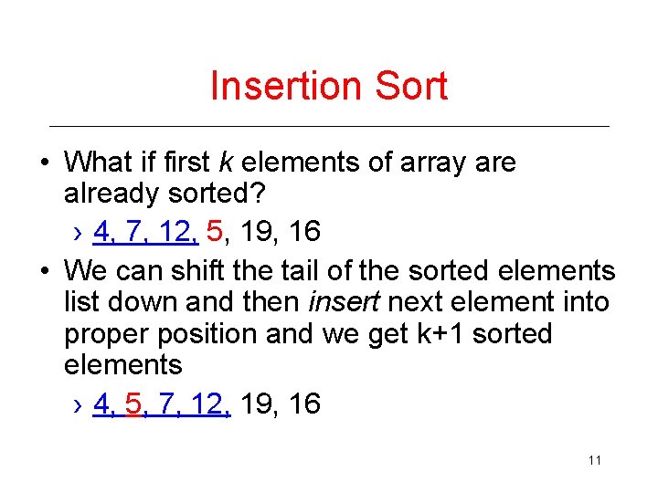
Insertion Sort • What if first k elements of array are already sorted? › 4, 7, 12, 5, 19, 16 • We can shift the tail of the sorted elements list down and then insert next element into proper position and we get k+1 sorted elements › 4, 5, 7, 12, 19, 16 11

Insertion Sort Insertion. Sort(A[1. . N]: integer array, N: integer) { i, j, temp: integer ; for i = 2 to N { temp : = A[i]; j : = i; while j > 1 and A[j-1] > temp { A[j] : = A[j-1]; j : = j– 1; } A[j] = temp; 1 2 3 } 2 1 4 } • Is Insertion sort in place? • Running time = ? i j 12

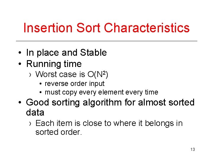
Insertion Sort Characteristics • In place and Stable • Running time › Worst case is O(N 2) • reverse order input • must copy every element every time • Good sorting algorithm for almost sorted data › Each item is close to where it belongs in sorted order. 13

Heap Sort • • We use a Max-Heap Root node = A[0] Children of A[i] = A[2 i+1], A[2 i+2] Keep track of current size N (number of nodes) value 7 5 6 2 4 index 0 1 2 3 4 7 5 5 6 7 2 6 4 N=5 14

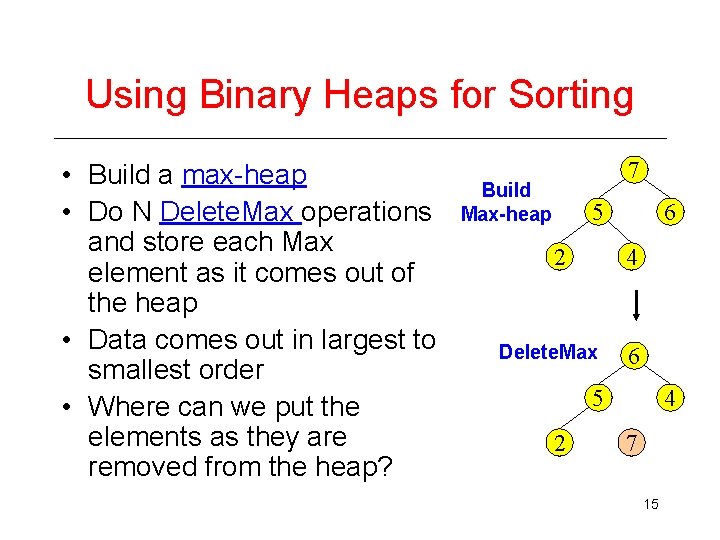
Using Binary Heaps for Sorting • Build a max-heap • Do N Delete. Max operations and store each Max element as it comes out of the heap • Data comes out in largest to smallest order • Where can we put the elements as they are removed from the heap? 7 Build Max-heap 5 2 6 4 Delete. Max 6 5 2 4 7 15

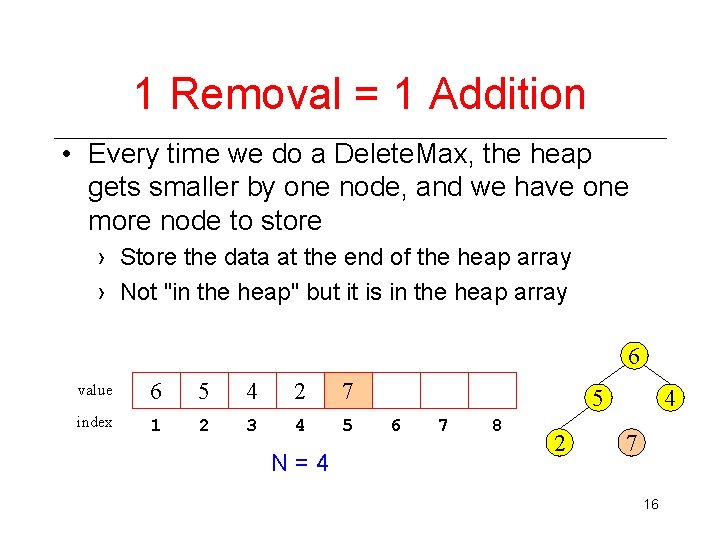
1 Removal = 1 Addition • Every time we do a Delete. Max, the heap gets smaller by one node, and we have one more node to store › Store the data at the end of the heap array › Not "in the heap" but it is in the heap array 6 value 6 5 4 2 7 index 1 2 3 4 5 N=4 5 6 7 8 2 4 7 16

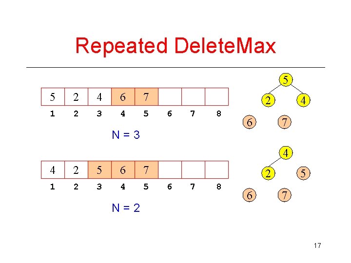
Repeated Delete. Max 5 5 2 4 6 7 1 2 3 4 5 2 6 7 8 N=3 6 4 7 4 4 2 5 6 7 1 2 3 4 5 N=2 2 6 7 8 6 5 7 17

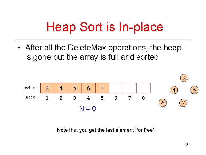
Heap Sort is In-place • After all the Delete. Max operations, the heap is gone but the array is full and sorted 2 value 2 4 5 6 7 index 1 2 3 4 5 4 6 7 8 N=0 6 5 7 Note that you get the last element ‘for free’ 18

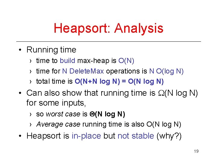
Heapsort: Analysis • Running time › time to build max-heap is O(N) › time for N Delete. Max operations is N O(log N) › total time is O(N+N log N) = O(N log N) • Can also show that running time is (N log N) for some inputs, › so worst case is (N log N) › Average case running time is also O(N log N) • Heapsort is in-place but not stable (why? ) 19

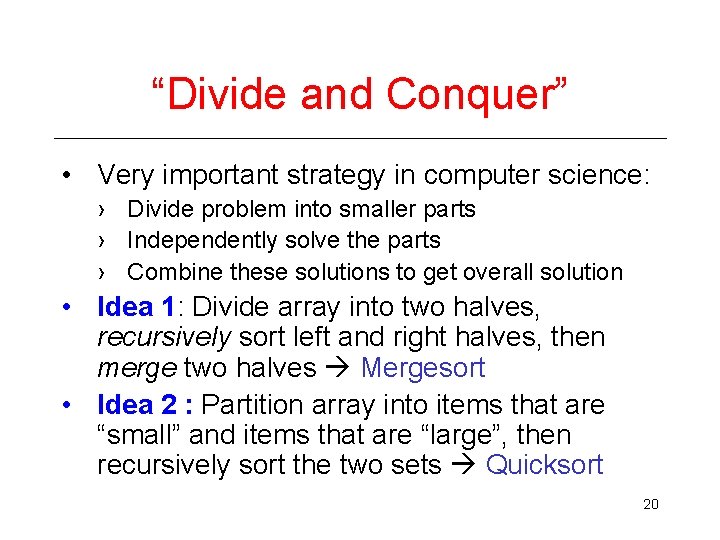
“Divide and Conquer” • Very important strategy in computer science: › Divide problem into smaller parts › Independently solve the parts › Combine these solutions to get overall solution • Idea 1: Divide array into two halves, recursively sort left and right halves, then merge two halves Mergesort • Idea 2 : Partition array into items that are “small” and items that are “large”, then recursively sort the two sets Quicksort 20

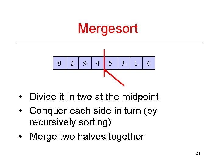
Mergesort 8 2 9 4 5 3 1 6 • Divide it in two at the midpoint • Conquer each side in turn (by recursively sorting) • Merge two halves together 21

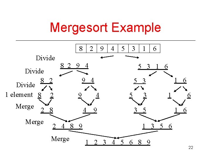
Mergesort Example 8 Divide 8 2 Divide 1 element 8 2 Merge 9 4 5 3 8 2 9 4 9 2 4 8 9 Merge 6 1 6 5 3 4 4 1 5 3 1 6 9 4 2 8 Merge 2 9 5 3 1 3 5 6 1 2 3 4 5 6 8 9 22

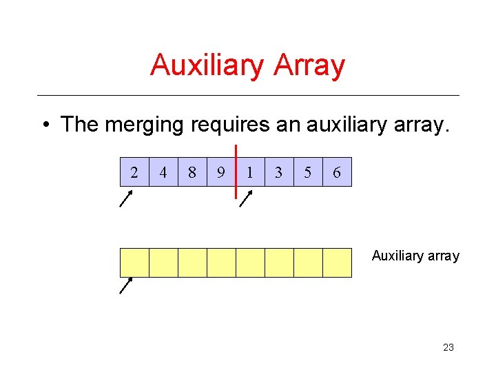
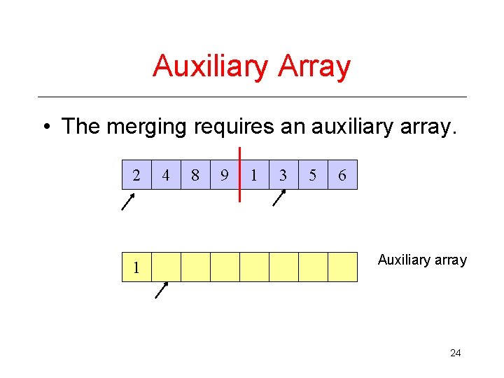
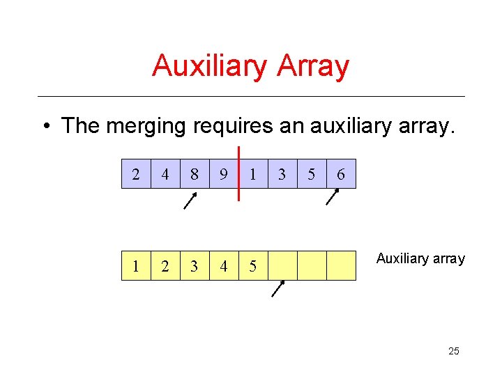
Auxiliary Array • The merging requires an auxiliary array. 2 4 8 9 1 3 5 6 Auxiliary array 23

Auxiliary Array • The merging requires an auxiliary array. 2 1 4 8 9 1 3 5 6 Auxiliary array 24

Auxiliary Array • The merging requires an auxiliary array. 2 4 8 9 1 1 2 3 4 5 3 5 6 Auxiliary array 25

Merging Algorithm Merge(A[], T[] : integer array, left, right : integer) : { mid, i, j, k, l, target : integer; mid : = (right + left)/2; i : = left; j : = mid + 1; target : = left; while i < mid and j < right do if A[i] < A[j] then T[target] : = A[i] ; i: = i + 1; else T[target] : = A[j]; j : = j + 1; target : = target + 1; if i > mid then //left completed// for k : = left to target-1 do A[k] : = T[k]; if j > right then //right completed// k : = mid; l : = right; while k > i do A[l] : = A[k]; k : = k-1; l : = l-1; for k : = left to target-1 do A[k] : = T[k]; } 26

Recursive Mergesort(A[], T[] : integer array, left, right : integer) : { if left < right then mid : = (left + right)/2; Mergesort(A, T, left, mid); Mergesort(A, T, mid+1, right); Merge(A, T, left, right); } Main. Mergesort(A[1. . n]: integer array, n : integer) : { T[1. . n]: integer array; Mergesort[A, T, 1, n]; } 27

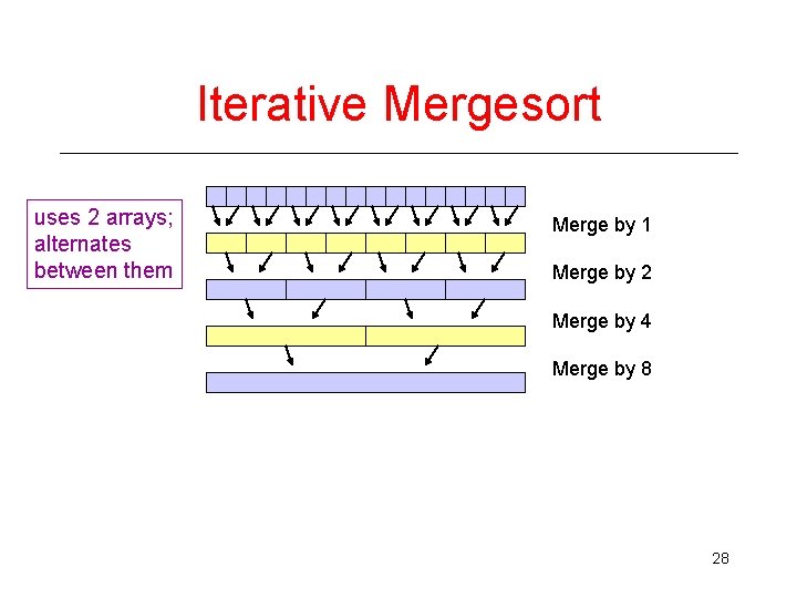
Iterative Mergesort uses 2 arrays; alternates between them Merge by 1 Merge by 2 Merge by 4 Merge by 8 28

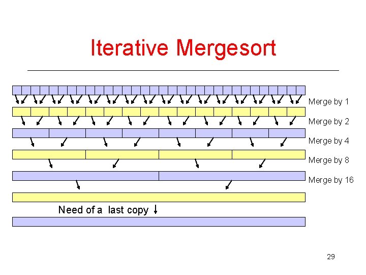
Iterative Mergesort Merge by 1 Merge by 2 Merge by 4 Merge by 8 Merge by 16 Need of a last copy 29

Iterative Mergesort Iterative. Mergesort(A[1. . n]: integer array, n : integer) : { //precondition: n is a power of 2// i, m, parity : integer; T[1. . n]: integer array; m : = 2; parity : = 0; while m < n do for i = 1 to n – m + 1 by m do if parity = 0 then Merge(A, T, i, i+m-1); else Merge(T, A, i, i+m-1); parity : = 1 – parity; m : = 2*m; if parity = 1 then for i = 1 to n do A[i] : = T[i]; } How do you handle non-powers of 2? How can the final copy be avoided? 30

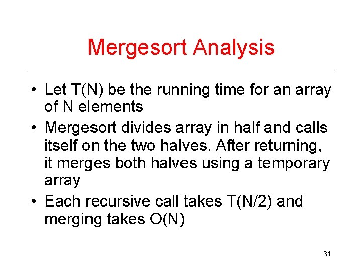
Mergesort Analysis • Let T(N) be the running time for an array of N elements • Mergesort divides array in half and calls itself on the two halves. After returning, it merges both halves using a temporary array • Each recursive call takes T(N/2) and merging takes O(N) 31

Properties of Mergesort • Not in-place › Requires an auxiliary array (O(n) extra space) • Stable › Only if left is sent to target on equal values. • Iterative Mergesort reduces copying. 32

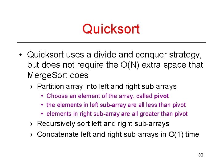
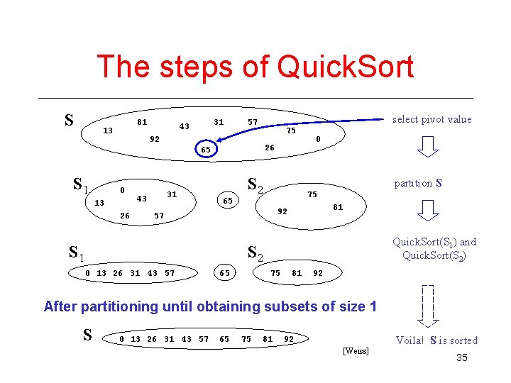
Quicksort • Quicksort uses a divide and conquer strategy, but does not require the O(N) extra space that Merge. Sort does › Partition array into left and right sub-arrays • Choose an element of the array, called pivot • the elements in left sub-array are all less than pivot • elements in right sub-array are all greater than pivot › Recursively sort left and right sub-arrays › Concatenate left and right sub-arrays in O(1) time 33

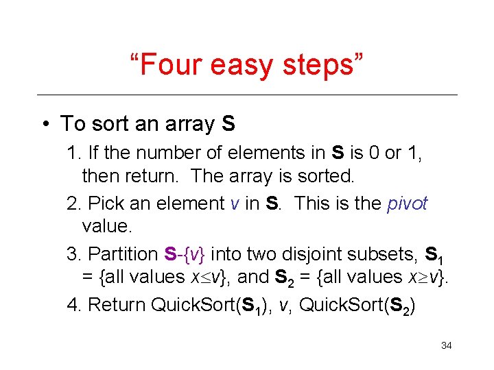
“Four easy steps” • To sort an array S 1. If the number of elements in S is 0 or 1, then return. The array is sorted. 2. Pick an element v in S. This is the pivot value. 3. Partition S-{v} into two disjoint subsets, S 1 = {all values x v}, and S 2 = {all values x v}. 4. Return Quick. Sort(S 1), v, Quick. Sort(S 2) 34

The steps of Quick. Sort S 81 13 31 43 select pivot value 57 75 92 26 65 S 1 0 13 26 31 43 S 2 0 partition S 75 65 81 92 57 S 1 Quick. Sort(S 1) and Quick. Sort(S 2) S 2 0 13 26 31 43 57 75 65 81 92 After partitioning until obtaining subsets of size 1 S 0 13 26 31 43 57 65 75 81 92 [Weiss] Voila! S is sorted 35

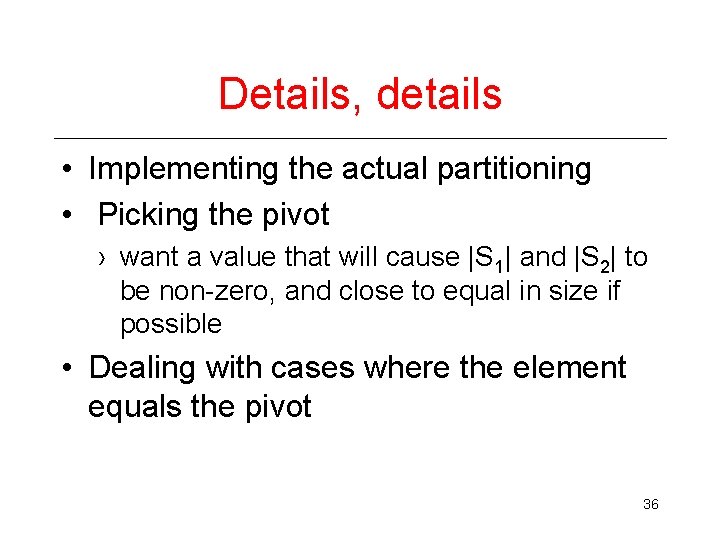
Details, details • Implementing the actual partitioning • Picking the pivot › want a value that will cause |S 1| and |S 2| to be non-zero, and close to equal in size if possible • Dealing with cases where the element equals the pivot 36

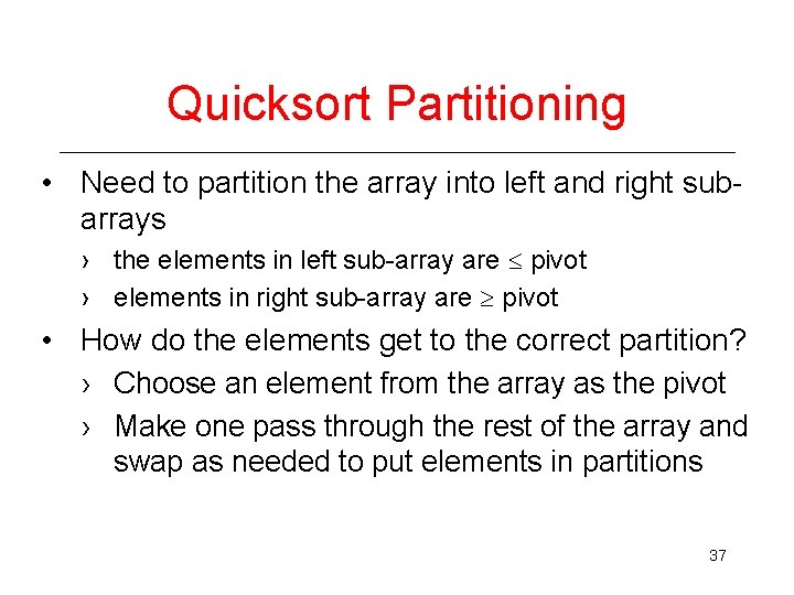
Quicksort Partitioning • Need to partition the array into left and right subarrays › the elements in left sub-array are pivot › elements in right sub-array are pivot • How do the elements get to the correct partition? › Choose an element from the array as the pivot › Make one pass through the rest of the array and swap as needed to put elements in partitions 37

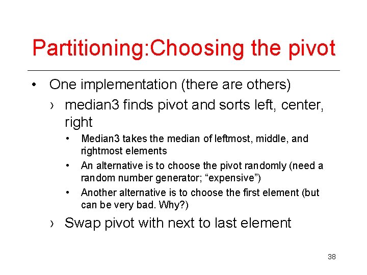
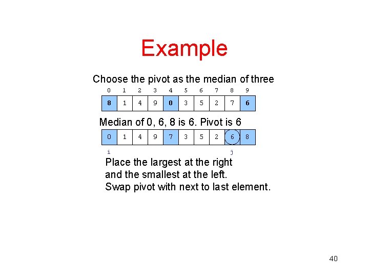
Partitioning: Choosing the pivot • One implementation (there are others) › median 3 finds pivot and sorts left, center, right • • • Median 3 takes the median of leftmost, middle, and rightmost elements An alternative is to choose the pivot randomly (need a random number generator; “expensive”) Another alternative is to choose the first element (but can be very bad. Why? ) › Swap pivot with next to last element 38

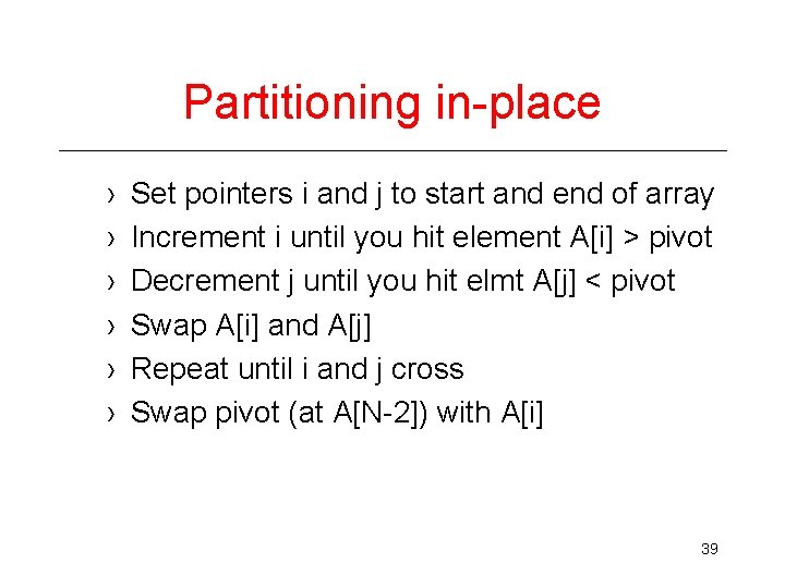
Partitioning in-place › › › Set pointers i and j to start and end of array Increment i until you hit element A[i] > pivot Decrement j until you hit elmt A[j] < pivot Swap A[i] and A[j] Repeat until i and j cross Swap pivot (at A[N-2]) with A[i] 39

Example Choose the pivot as the median of three 0 1 2 3 4 5 6 7 8 9 8 1 4 9 0 3 5 2 7 6 Median of 0, 6, 8 is 6. Pivot is 6 0 i 1 4 9 7 3 5 2 6 8 j Place the largest at the right and the smallest at the left. Swap pivot with next to last element. 40

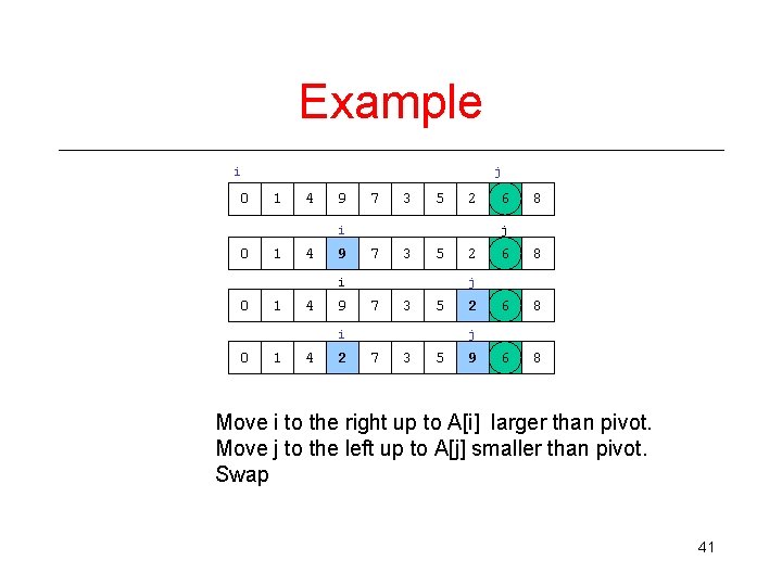
Example i 0 j 1 4 9 7 3 5 2 i 0 1 4 9 7 3 5 1 4 2 2 6 8 6 8 j 7 3 5 i 0 8 j i 0 6 2 j 7 3 5 9 Move i to the right up to A[i] larger than pivot. Move j to the left up to A[j] smaller than pivot. Swap 41

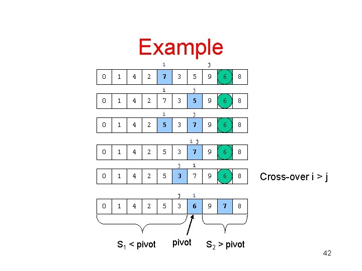
Example i 0 1 4 2 7 j 3 5 i 0 1 4 2 7 1 4 2 5 6 8 9 6 8 9 7 8 j 3 5 i 0 9 j 3 7 i j 0 0 0 1 1 1 4 4 4 2 2 2 S 1 < pivot 5 5 5 3 7 j i 3 6 pivot S 2 > pivot Cross-over i > j 42

Recursive Quicksort(A[]: integer array, left, right : integer): { pivotindex : integer; if left + CUTOFF right then pivot : = median 3(A, left, right); pivotindex : = Partition(A, left, right-1, pivot); Quicksort(A, left, pivotindex – 1); Quicksort(A, pivotindex + 1, right); else Insertionsort(A, left, right); } Don’t use quicksort for small arrays. CUTOFF = 10 is reasonable. 43

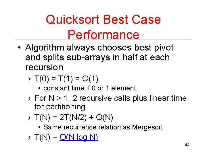
Quicksort Best Case Performance • Algorithm always chooses best pivot and splits sub-arrays in half at each recursion › T(0) = T(1) = O(1) • constant time if 0 or 1 element › For N > 1, 2 recursive calls plus linear time for partitioning › T(N) = 2 T(N/2) + O(N) • Same recurrence relation as Mergesort › T(N) = O(N log N) 44

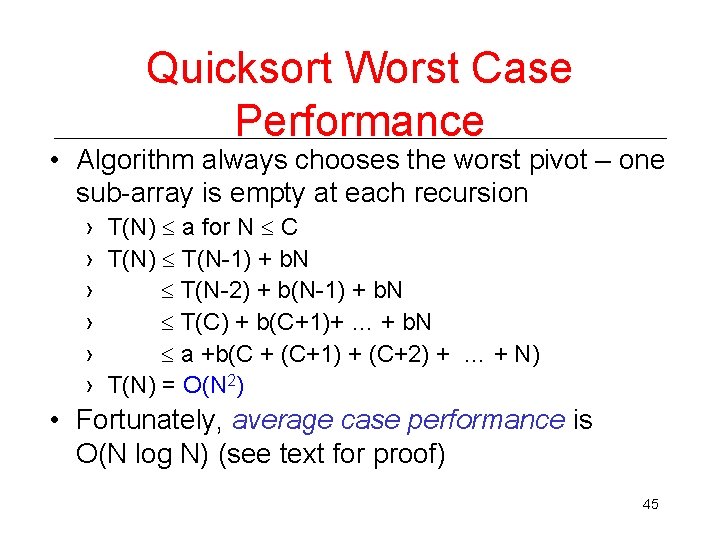
Quicksort Worst Case Performance • Algorithm always chooses the worst pivot – one sub-array is empty at each recursion › T(N) a for N C › T(N) T(N-1) + b. N › T(N-2) + b(N-1) + b. N › T(C) + b(C+1)+ … + b. N › a +b(C + (C+1) + (C+2) + … + N) › T(N) = O(N 2) • Fortunately, average case performance is O(N log N) (see text for proof) 45

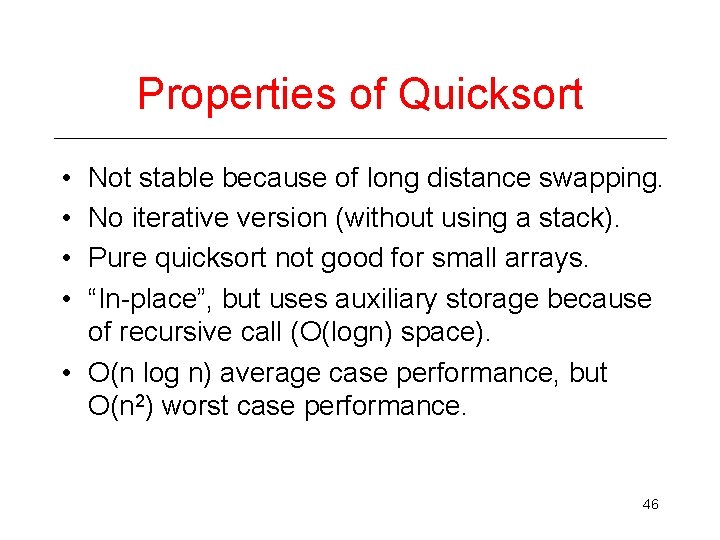
Properties of Quicksort • • Not stable because of long distance swapping. No iterative version (without using a stack). Pure quicksort not good for small arrays. “In-place”, but uses auxiliary storage because of recursive call (O(logn) space). • O(n log n) average case performance, but O(n 2) worst case performance. 46

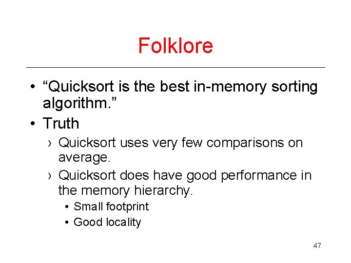
Folklore • “Quicksort is the best in-memory sorting algorithm. ” • Truth › Quicksort uses very few comparisons on average. › Quicksort does have good performance in the memory hierarchy. • Small footprint • Good locality 47