Sorting Cont Quick Sort As the name implies

Sorting Cont

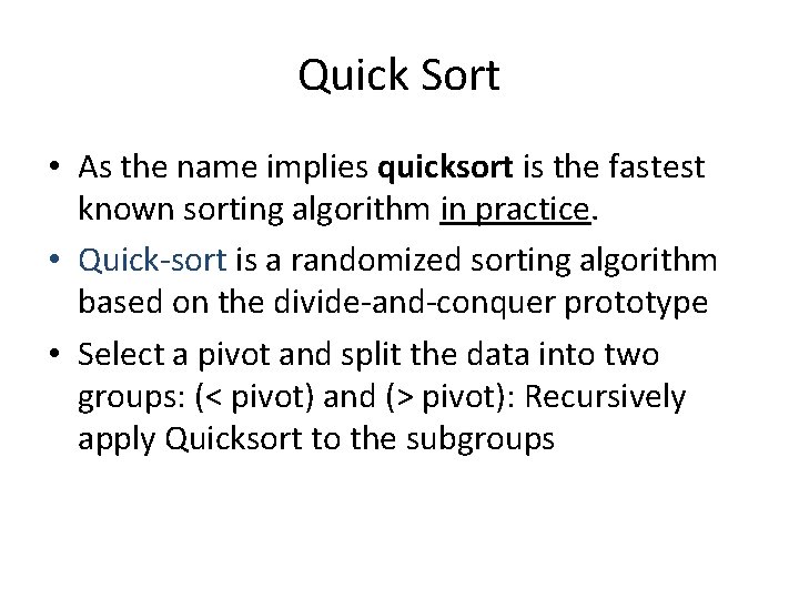
Quick Sort • As the name implies quicksort is the fastest known sorting algorithm in practice. • Quick-sort is a randomized sorting algorithm based on the divide-and-conquer prototype • Select a pivot and split the data into two groups: (< pivot) and (> pivot): Recursively apply Quicksort to the subgroups

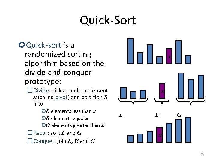
Quick-Sort Quick-sort is a randomized sorting algorithm based on the divide-and-conquer prototype: x � Divide: pick a random element x (called pivot) and partition S into L elements less than x E elements equal x G elements greater than x � Recur: sort L and G � Conquer: join L, E and G x L E G x 3

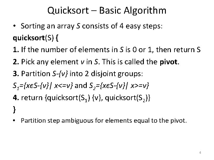
Quicksort – Basic Algorithm • Sorting an array S consists of 4 easy steps: quicksort(S) { 1. If the number of elements in S is 0 or 1, then return S 2. Pick any element v in S. This is called the pivot. 3. Partition S-{v} into 2 disjoint groups: S 1={xєS-{v}| x<=v} and S 2={xєS-{v}| x>=v} 4. return {quicksort(S 1) {v}, quicksort(S 2)} } • Partition step ambiguous for elements equal to the pivot. 4

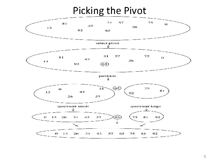
Picking the Pivot 5

Quicksort Start with all data in an array, and consider it unsorted Unsorted Array

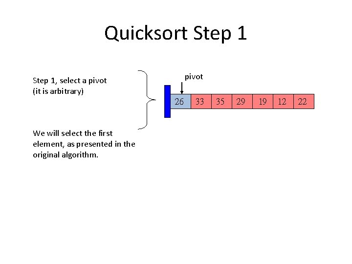
Quicksort Step 1 pivot Step 1, select a pivot (it is arbitrary) 26 We will select the first element, as presented in the original algorithm. 33 35 29 19 12 22

Quicksort Step 2, start process of dividing data into LEFT and RIGHT groups: The LEFT group will have elements less than the pivot. The RIGHT group will have elements greater that the pivot. Use markers left and right pivot 26 33 left 35 29 19 12 22 right

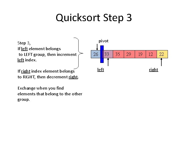
Quicksort Step 3, If left element belongs to LEFT group, then increment left index. If right index element belongs to RIGHT, then decrement right. Exchange when you find elements that belong to the other group. pivot 26 left 33 35 29 19 12 right 22

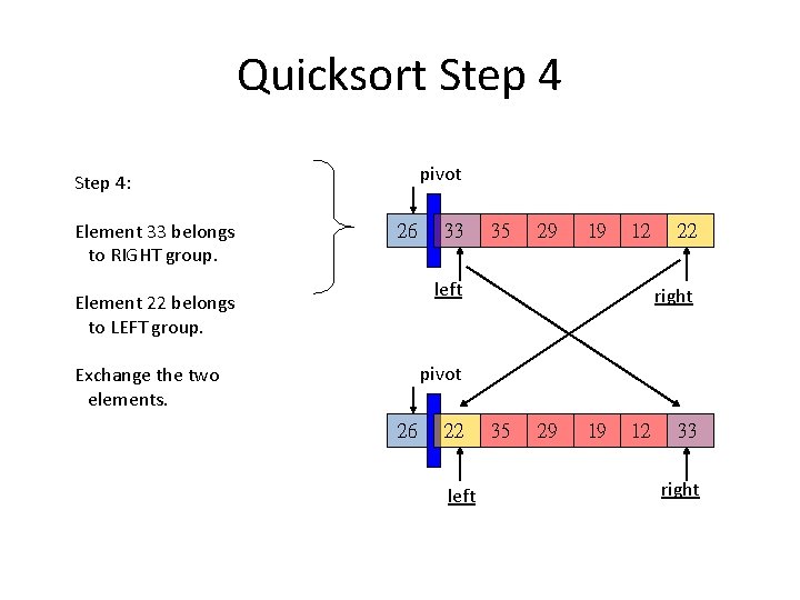
Quicksort Step 4 pivot Step 4: Element 33 belongs to RIGHT group. 26 33 35 29 19 12 left Element 22 belongs to LEFT group. 22 right pivot Exchange the two elements. 26 22 left 35 29 19 12 33 right

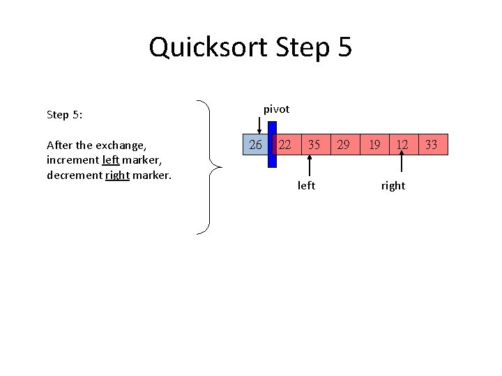
Quicksort Step 5 pivot Step 5: After the exchange, increment left marker, decrement right marker. 26 22 35 left 29 19 12 right 33

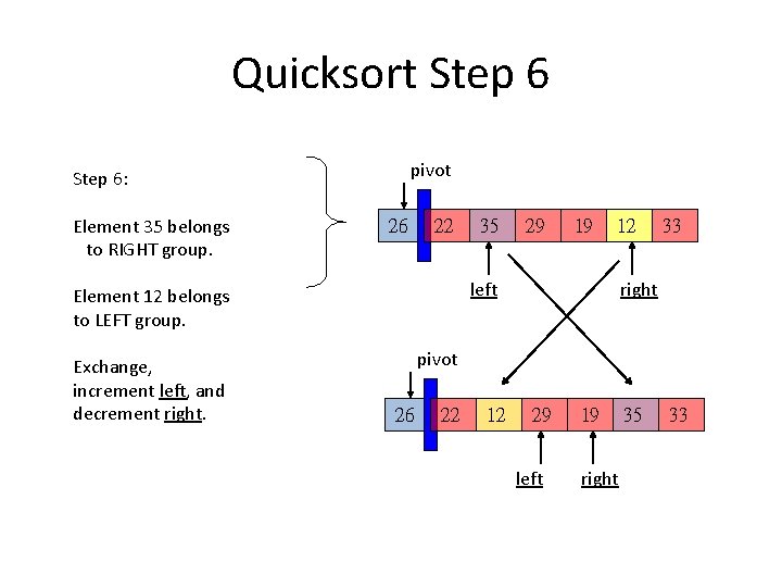
Quicksort Step 6 pivot Step 6: Element 35 belongs to RIGHT group. 26 22 29 19 12 left Element 12 belongs to LEFT group. Exchange, increment left, and decrement right. 35 33 right pivot 26 22 12 29 left 19 right 35 33

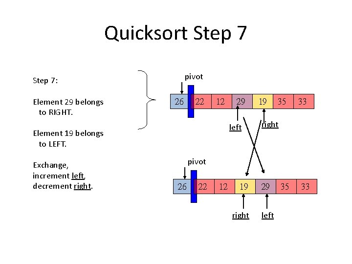
Quicksort Step 7 pivot Step 7: Element 29 belongs to RIGHT. 26 22 12 left Element 19 belongs to LEFT. Exchange, increment left, decrement right. 29 19 35 33 right pivot 26 22 12 19 right 29 left 35 33

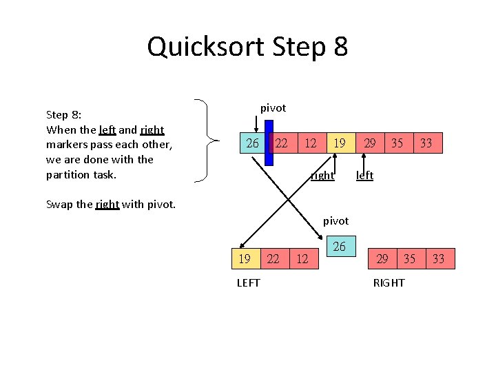
Quicksort Step 8: When the left and right markers pass each other, we are done with the partition task. pivot 26 22 12 19 right 29 35 33 left Swap the right with pivot 26 19 LEFT 22 12 29 35 RIGHT 33

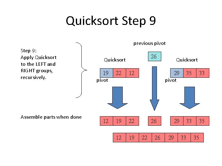
Quicksort Step 9 previous pivot Step 9: Apply Quicksort to the LEFT and RIGHT groups, recursively. Assemble parts when done 26 Quicksort 19 pivot 22 12 12 19 22 12 19 Quicksort 29 pivot 35 33 29 33 35 26 22 26 29 33 35

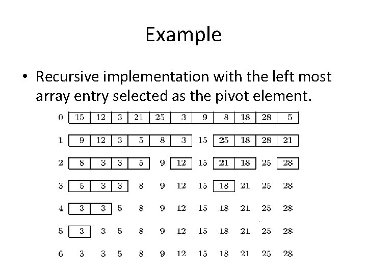
Example • Recursive implementation with the left most array entry selected as the pivot element.

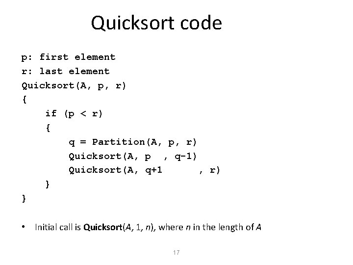
Quicksort code p: first element r: last element Quicksort(A, p, r) { if (p < r) { q = Partition(A, p, r) Quicksort(A, p , q-1) Quicksort(A, q+1 , r) } } • Initial call is Quicksort(A, 1, n), where n in the length of A 17

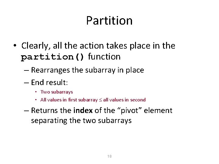
Partition • Clearly, all the action takes place in the partition() function – Rearranges the subarray in place – End result: • Two subarrays • All values in first subarray all values in second – Returns the index of the “pivot” element separating the two subarrays 18

Partition Code Partition(A, p, r) { x = A[r] // x is pivot i = p - 1 for j = p to r – 1 { do if A[j] <= x then { i = i + 1 exchange A[i] A[j] } } exchange A[i+1] A[r] return i+1 } 19

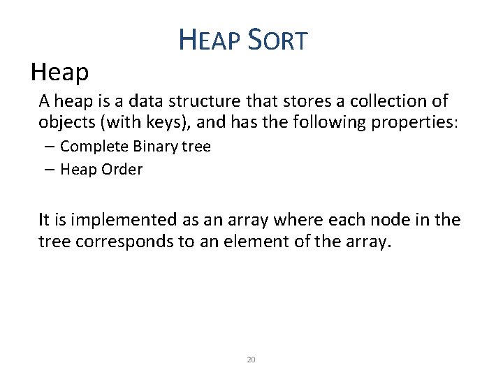
Heap HEAP SORT A heap is a data structure that stores a collection of objects (with keys), and has the following properties: – Complete Binary tree – Heap Order It is implemented as an array where each node in the tree corresponds to an element of the array. 20

Binary Tree • a binary tree is a tree data structure in which each node has at most two children (referred to as the left child and the right child). • In a binary tree, the degree of each node can be at most two. Binary trees are used to implement binary search and heap sort Parent node Left child node 5 4 3 Right child node

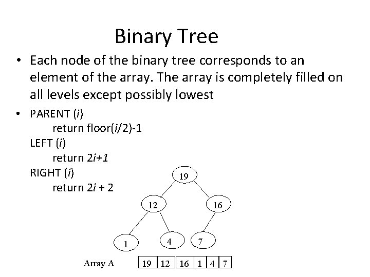
Binary Tree • Each node of the binary tree corresponds to an element of the array. The array is completely filled on all levels except possibly lowest • PARENT (i) return floor(i/2)-1 LEFT (i) return 2 i+1 RIGHT (i) return 2 i + 2 19 12 4 1 Array A 16 19 12 7 16 1 4 7

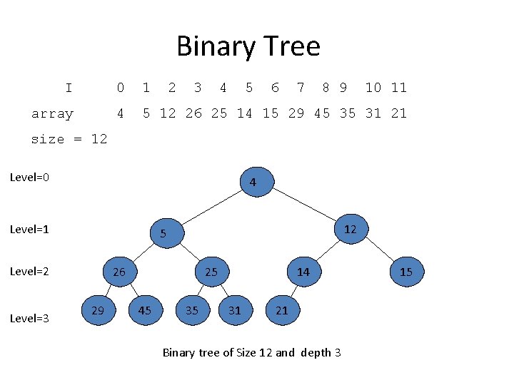
Binary Tree I 0 1 2 3 4 5 6 7 8 9 10 11 array 4 5 12 26 25 14 15 29 45 35 31 21 size = 12 Level=0 4 Level=1 Level=2 Level=3 12 5 26 29 25 45 35 14 31 21 Binary tree of Size 12 and depth 3 15

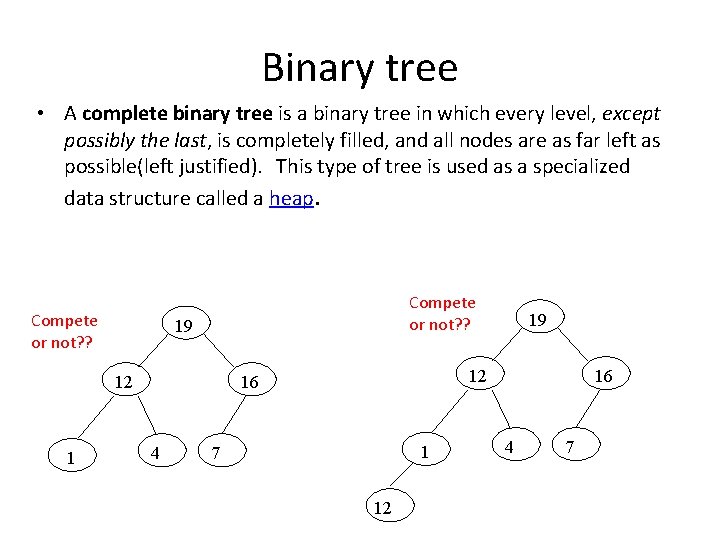
Binary tree • A complete binary tree is a binary tree in which every level, except possibly the last, is completely filled, and all nodes are as far left as possible(left justified). This type of tree is used as a specialized data structure called a heap. Compete or not? ? 19 12 16 4 19 1 7 12 16 4 7

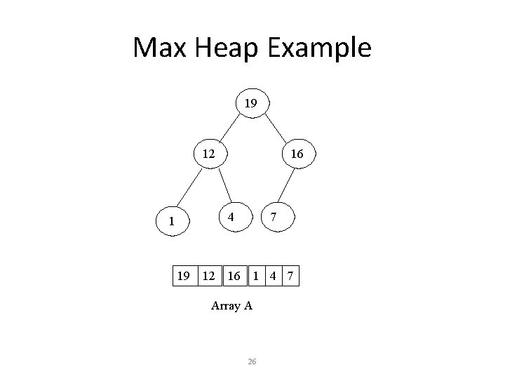
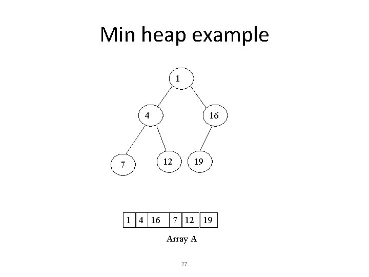
What is a Binary Heap? • A binary heap is a complete binary tree with one (or both) of the following heap order properties: • Min. Heap property: Each node must have a key that is less or equal to the key of each of its children. • Max. Heap property: Each node must have a key that is greater or equal to the key of each of its children. • A binary heap satisfying the Min. Heap property is called a Min. Heap. • A binary heap satisfying the Max. Heap property is called a Max. Heap. • Recall: A complete binary tree may have missing nodes only on the right side of the lowest level.

Max Heap Example 19 12 16 4 7 16 1 4 7 Array A 26

Min heap example 1 4 16 12 7 1 4 16 19 7 12 Array A 27 19

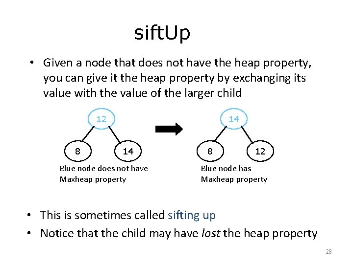
sift. Up • Given a node that does not have the heap property, you can give it the heap property by exchanging its value with the value of the larger child 12 8 14 14 Blue node does not have Maxheap property 8 12 Blue node has Maxheap property • This is sometimes called sifting up • Notice that the child may have lost the heap property 28

Plan of attack • First, we will learn how to turn a binary tree into a heap • Next, we will learn how to turn a binary tree back into a heap after it has been changed in a certain way • Finally (this is the cool part) we will see how to use these ideas to sort an array 29

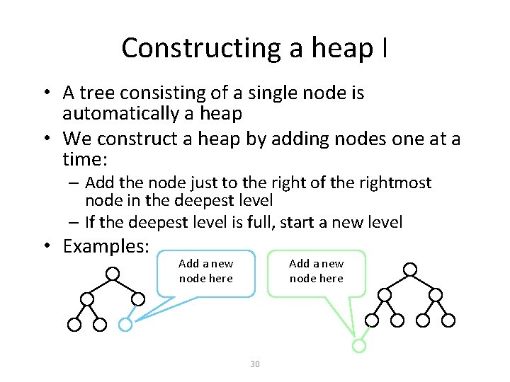
Constructing a heap I • A tree consisting of a single node is automatically a heap • We construct a heap by adding nodes one at a time: – Add the node just to the right of the rightmost node in the deepest level – If the deepest level is full, start a new level • Examples: Add a new node here 30

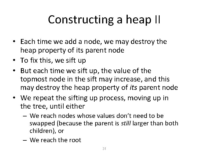
Constructing a heap II • Each time we add a node, we may destroy the heap property of its parent node • To fix this, we sift up • But each time we sift up, the value of the topmost node in the sift may increase, and this may destroy the heap property of its parent node • We repeat the sifting up process, moving up in the tree, until either – We reach nodes whose values don’t need to be swapped (because the parent is still larger than both children), or – We reach the root 31

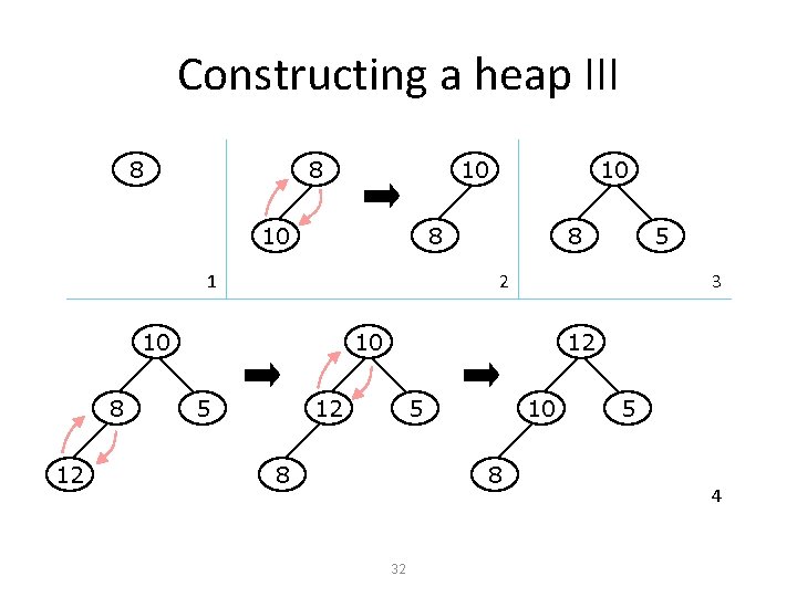
Constructing a heap III 8 8 10 10 8 1 12 8 5 2 10 8 10 3 10 5 12 12 5 8 10 8 32 5 4

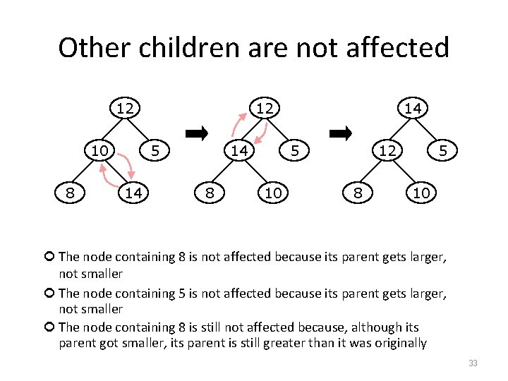
Other children are not affected 12 10 8 12 5 14 14 8 14 5 10 12 8 5 10 The node containing 8 is not affected because its parent gets larger, not smaller The node containing 5 is not affected because its parent gets larger, not smaller The node containing 8 is still not affected because, although its parent got smaller, its parent is still greater than it was originally 33

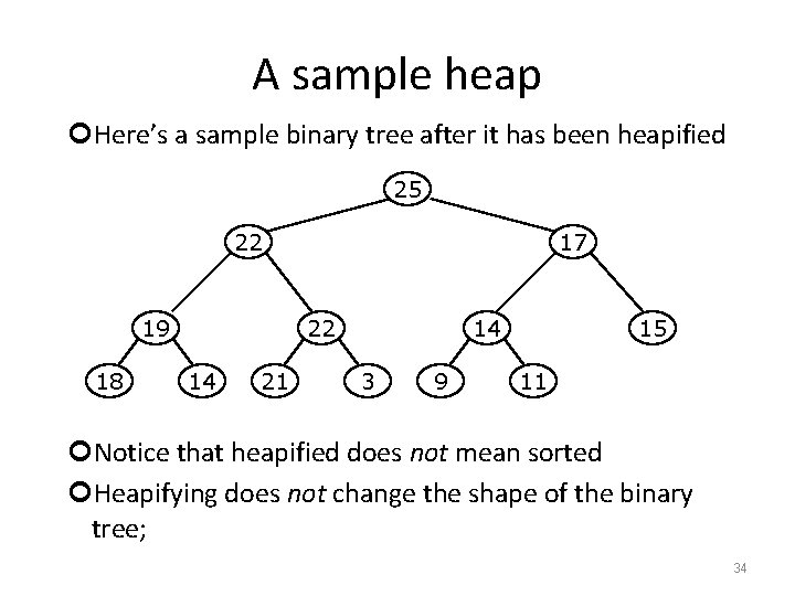
A sample heap Here’s a sample binary tree after it has been heapified 25 22 19 18 17 22 14 21 14 3 9 15 11 Notice that heapified does not mean sorted Heapifying does not change the shape of the binary tree; 34

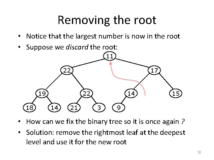
Removing the root • Notice that the largest number is now in the root • Suppose we discard the root: 11 22 19 18 17 22 14 21 14 3 9 15 11 • How can we fix the binary tree so it is once again ? • Solution: remove the rightmost leaf at the deepest level and use it for the new root 35

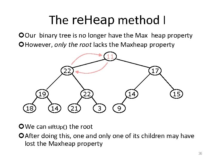
The re. Heap method I Our binary tree is no longer have the Max heap property However, only the root lacks the Maxheap property 11 22 19 18 17 22 14 21 14 3 15 9 We can sift. Up() the root After doing this, one and only one of its children may have lost the Maxheap property 36

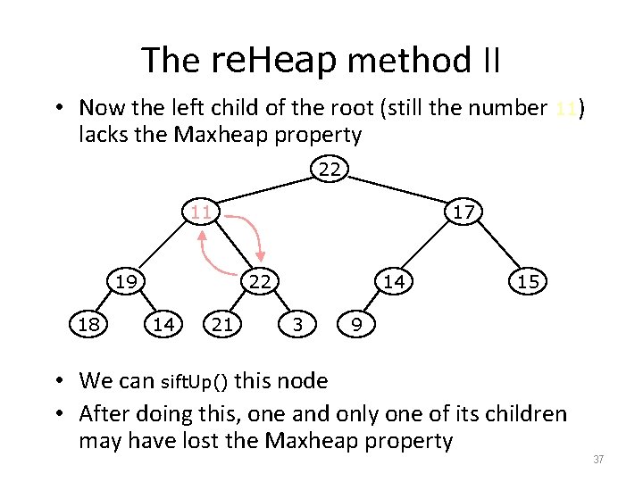
The re. Heap method II • Now the left child of the root (still the number 11) lacks the Maxheap property 22 11 19 18 17 22 14 21 14 3 15 9 • We can sift. Up() this node • After doing this, one and only one of its children may have lost the Maxheap property 37

The re. Heap method III Now the right child of the left child of the root (still the number 11) lacks the Maxheap property: 22 22 19 18 17 11 14 21 14 3 15 9 We can sift. Up() this node After doing this, one and only one of its children may have lost the Maxheap property —but it doesn’t, because it’s a leaf 38

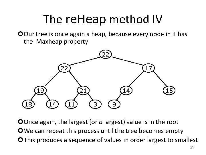
The re. Heap method IV Our tree is once again a heap, because every node in it has the Maxheap property 22 22 19 18 17 21 14 11 14 3 15 9 Once again, the largest (or a largest) value is in the root We can repeat this process until the tree becomes empty This produces a sequence of values in order largest to smallest 39

Sorting • What do heaps have to do with sorting an array? • Here’s the neat part: – Because the compete binary tree can be represented as an array – All our operations on the complete binary trees can be represented as operations on arrays – To sort: heapify the array; while the array isn’t empty { remove and replace the root; reheap the new root node; } 40

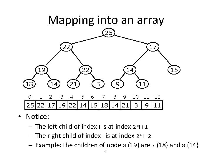
Mapping into an array 25 22 17 19 18 0 22 14 1 2 14 21 3 4 3 5 6 9 7 8 15 11 9 10 25 22 17 19 22 14 15 18 14 21 3 11 12 9 11 • Notice: – The left child of index i is at index 2*i+1 – The right child of index i is at index 2*i+2 – Example: the children of node 3 (19) are 7 (18) and 8 (14) 41

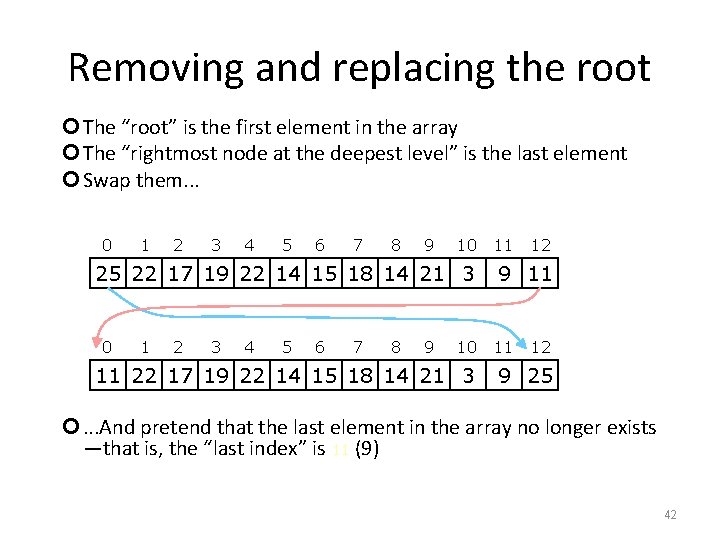
Removing and replacing the root The “root” is the first element in the array The “rightmost node at the deepest level” is the last element Swap them. . . 0 1 2 3 4 5 6 7 8 9 10 25 22 17 19 22 14 15 18 14 21 3 0 1 2 3 4 5 6 7 8 9 10 11 22 17 19 22 14 15 18 14 21 3 11 12 9 11 11 12 9 25 . . . And pretend that the last element in the array no longer exists —that is, the “last index” is 11 (9) 42

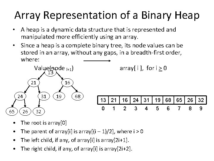
Array Representation of a Binary Heap • A heap is a dynamic data structure that is represented and manipulated more efficiently using an array. • Since a heap is a complete binary tree, its node values can be stored in an array, without any gaps, in a breadth-first order, where: Value(node i+1) array[ i ], for i > 0 13 21 24 65 • • 26 16 31 32 19 68 13 21 16 24 31 19 68 65 26 32 0 1 2 3 The root is array[0] The parent of array[i] is array[(i – 1)/2], where i > 0 The left child, if any, of array[i] is array[2 i+1]. The right child, if any, of array[i] is array[2 i+2]. 4 5 6 7 8 9

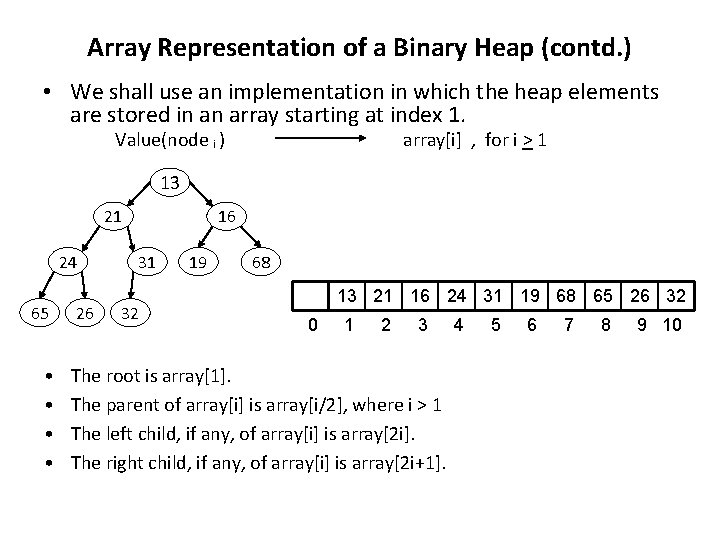
Array Representation of a Binary Heap (contd. ) • We shall use an implementation in which the heap elements are stored in an array starting at index 1. Value(node i ) array[i] , for i > 1 13 21 24 65 • • 26 16 31 32 19 68 13 21 16 24 31 19 68 65 26 32 0 1 2 3 The root is array[1]. The parent of array[i] is array[i/2], where i > 1 The left child, if any, of array[i] is array[2 i]. The right child, if any, of array[i] is array[2 i+1]. 4 5 6 7 8 9 10

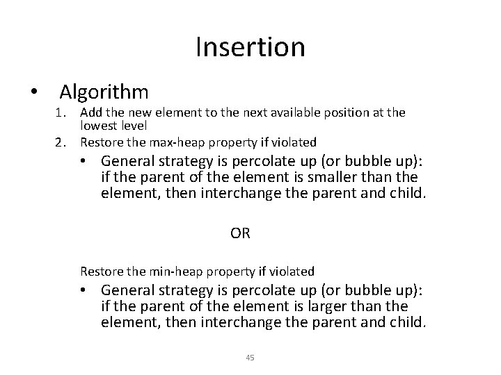
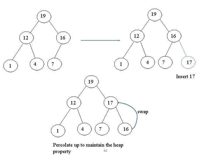
Insertion • Algorithm 1. Add the new element to the next available position at the lowest level 2. Restore the max-heap property if violated • General strategy is percolate up (or bubble up): if the parent of the element is smaller than the element, then interchange the parent and child. OR Restore the min-heap property if violated • General strategy is percolate up (or bubble up): if the parent of the element is larger than the element, then interchange the parent and child. 45

19 19 12 16 4 7 16 4 1 12 17 swap 4 17 Insert 17 19 1 7 7 16 Percolate up to maintain the heap 46 property

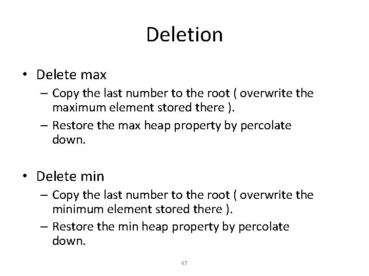
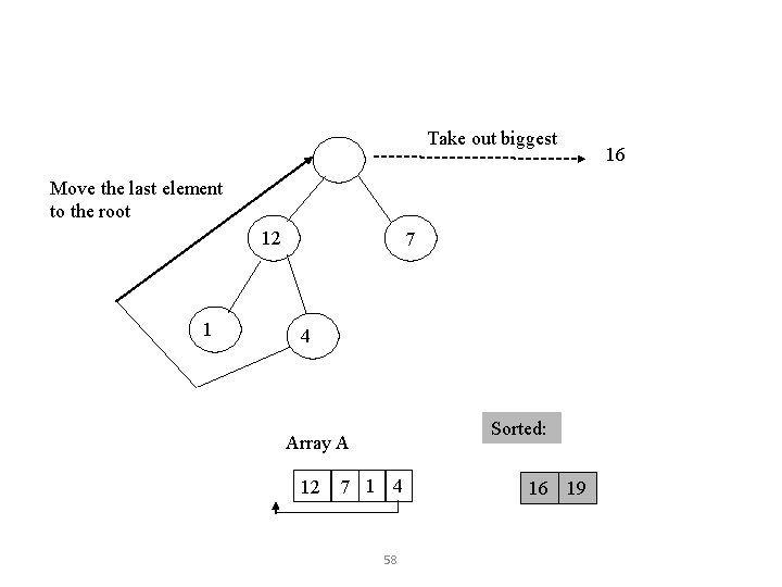
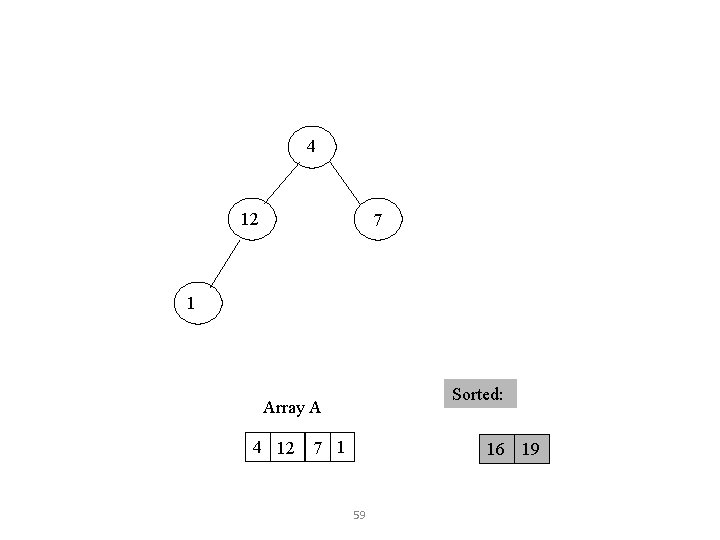
Deletion • Delete max – Copy the last number to the root ( overwrite the maximum element stored there ). – Restore the max heap property by percolate down. • Delete min – Copy the last number to the root ( overwrite the minimum element stored there ). – Restore the min heap property by percolate down. 47

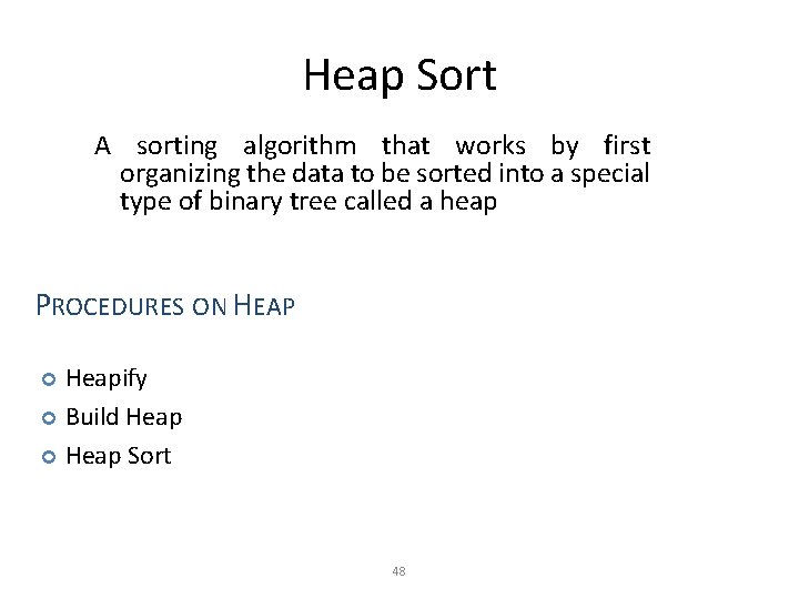
Heap Sort A sorting algorithm that works by first organizing the data to be sorted into a special type of binary tree called a heap PROCEDURES ON HEAP Heapify Build Heap Sort 48

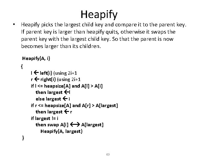
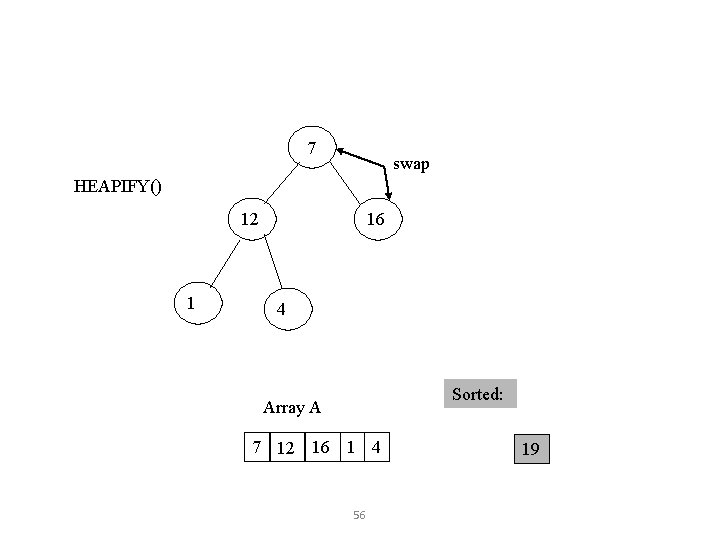
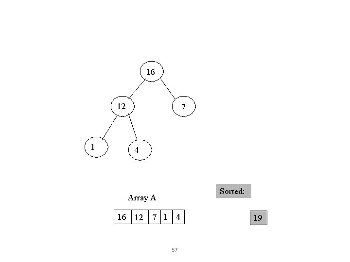
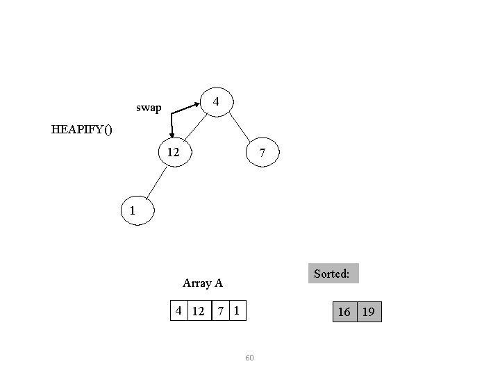
Heapify • Heapify picks the largest child key and compare it to the parent key. If parent key is larger than heapify quits, otherwise it swaps the parent key with the largest child key. So that the parent is now becomes larger than its children. Heapify(A, i) { } l left(i) (using 2 i+1 r right(i) (using 2 i+1 if l <= heapsize[A] and A[l] > A[i] then largest l else largest i if r <= heapsize[A] and A[r] > A[largest] then largest r if largest != i then swap A[i] A[largest] Heapify(A, largest) 49

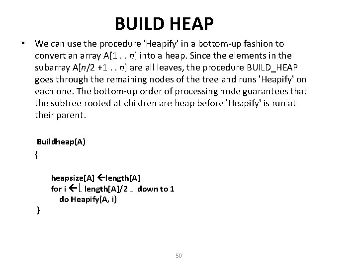
BUILD HEAP • We can use the procedure 'Heapify' in a bottom-up fashion to convert an array A[1. . n] into a heap. Since the elements in the subarray A[n/2 +1. . n] are all leaves, the procedure BUILD_HEAP goes through the remaining nodes of the tree and runs 'Heapify' on each one. The bottom-up order of processing node guarantees that the subtree rooted at children are heap before 'Heapify' is run at their parent. Buildheap(A) { } heapsize[A] length[A] for i length[A]/2 down to 1 do Heapify(A, i) 50

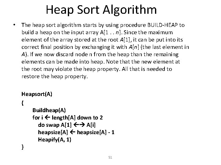
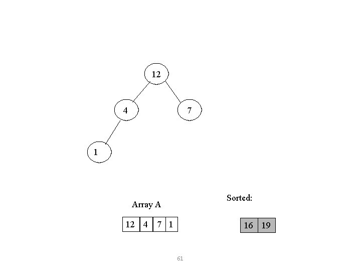
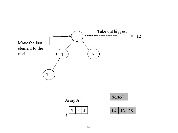
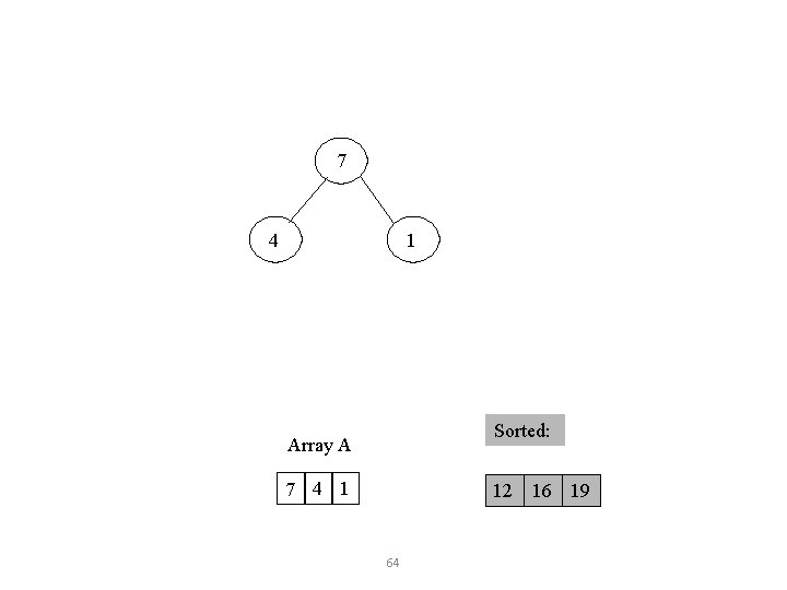
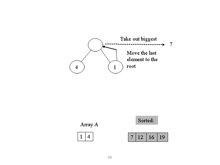
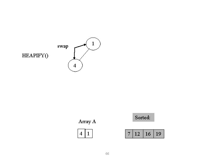
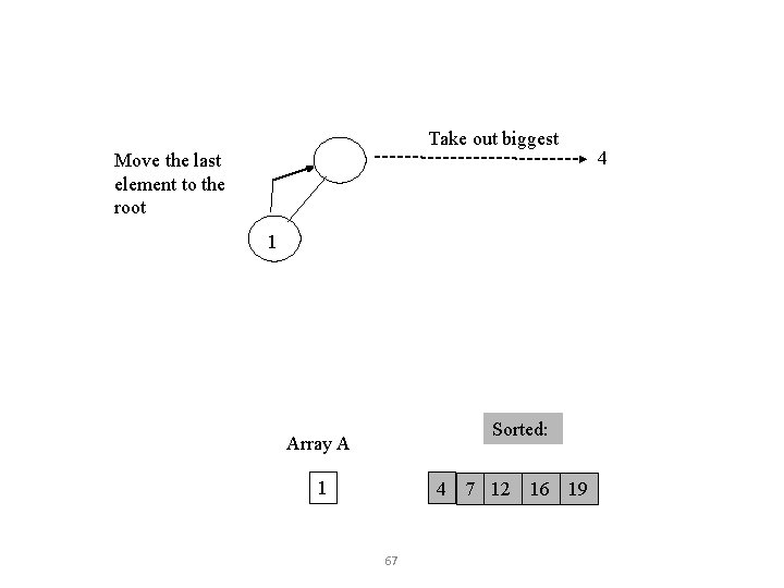
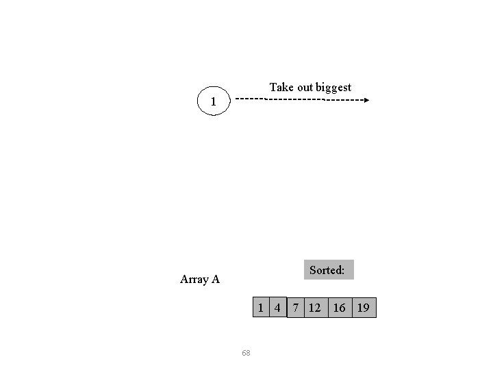
Heap Sort Algorithm • The heap sort algorithm starts by using procedure BUILD-HEAP to build a heap on the input array A[1. . n]. Since the maximum element of the array stored at the root A[1], it can be put into its correct final position by exchanging it with A[n] (the last element in A). If we now discard node n from the heap than the remaining elements can be made into heap. Note that the new element at the root may violate the heap property. All that is needed to restore the heap property. Heapsort(A) { Buildheap(A) for i length[A] down to 2 do swap A[1] A[i] heapsize[A] - 1 Heapify(A, 1) } 51

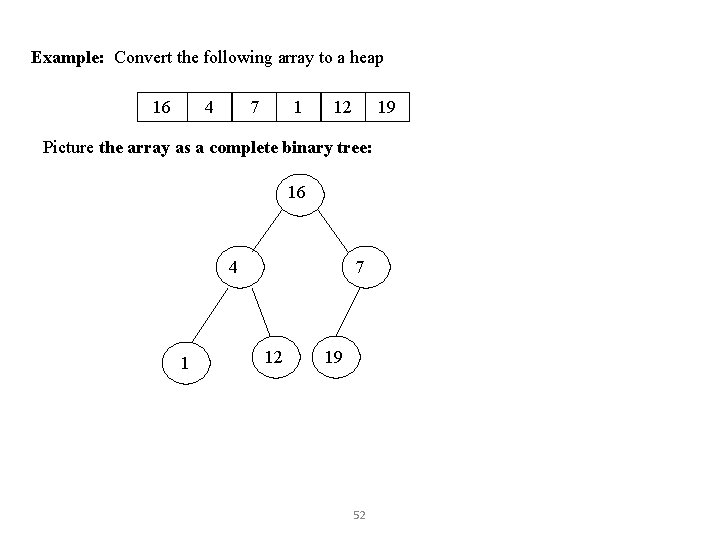
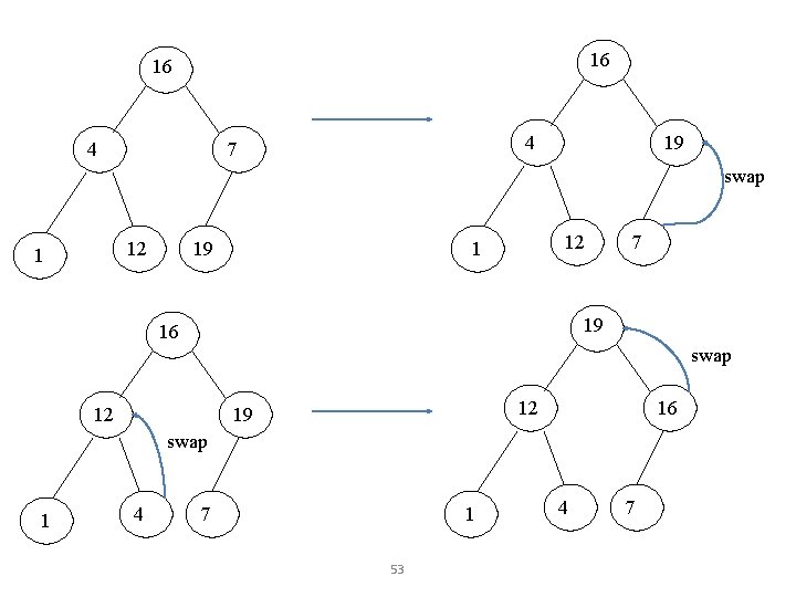
Example: Convert the following array to a heap 16 4 7 1 12 19 Picture the array as a complete binary tree: 16 4 1 7 12 19 52

16 16 4 4 7 19 swap 12 1 19 12 1 7 19 16 swap 12 12 19 16 swap 1 4 7 1 53 4 7

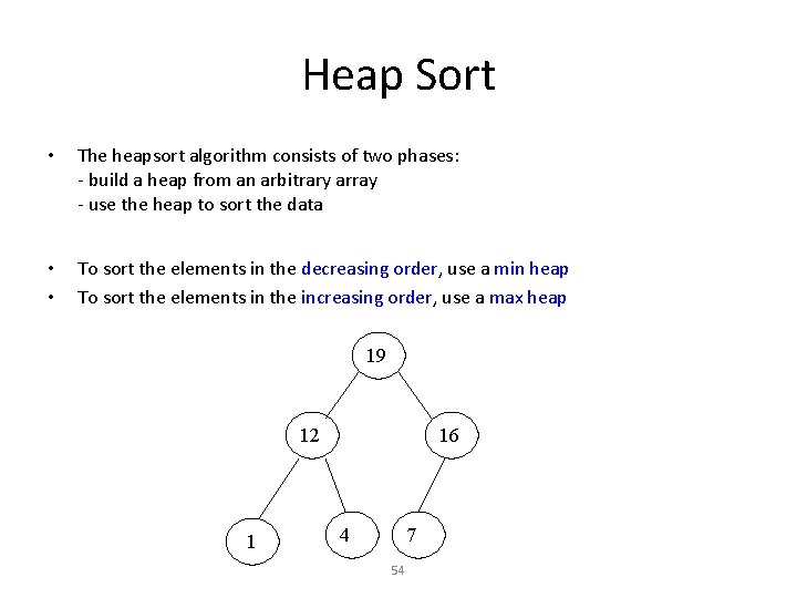
Heap Sort • The heapsort algorithm consists of two phases: - build a heap from an arbitrary array - use the heap to sort the data • • To sort the elements in the decreasing order, use a min heap To sort the elements in the increasing order, use a max heap 19 12 1 16 4 7 54

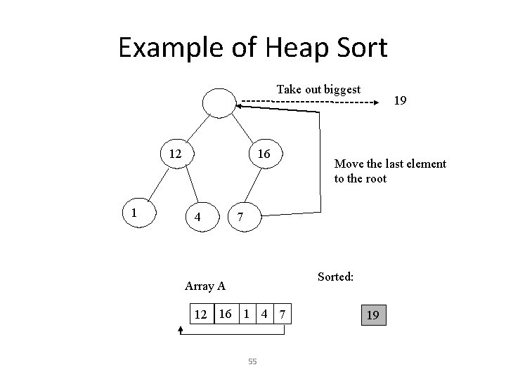
Example of Heap Sort Take out biggest 12 1 16 4 19 Move the last element to the root 7 Sorted: Array A 12 16 1 4 7 55 19

7 swap HEAPIFY() 12 1 16 4 Sorted: Array A 7 12 16 1 4 56 19

16 12 1 7 4 Sorted: Array A 16 12 7 1 4 57 19

Take out biggest Move the last element to the root 12 1 7 4 Sorted: Array A 12 7 1 4 58 16 19 16

4 12 7 1 Sorted: Array A 4 12 7 1 16 19 59

4 swap HEAPIFY() 12 7 1 Sorted: Array A 4 12 7 1 16 19 60

12 7 4 1 Sorted: Array A 12 4 7 1 16 19 61

Take out biggest Move the last element to the root 7 4 1 Sorted: Array A 4 7 1 12 16 19 62 12

1 swap 7 4 Sorted: Array A 1 4 7 12 16 19 63

7 4 1 Sorted: Array A 7 4 1 12 16 19 64

Take out biggest 4 1 Move the last element to the root Sorted: Array A 1 4 7 12 16 19 65 7

1 swap HEAPIFY() 4 Sorted: Array A 4 1 7 12 16 19 66

Take out biggest Move the last element to the root 1 Sorted: Array A 1 4 7 12 16 19 67 4

Take out biggest 1 Sorted: Array A 1 4 7 12 16 19 68