Sorting and Searching Bubble Sort Linear Search Binary

Sorting and Searching Bubble Sort Linear Search Binary Search

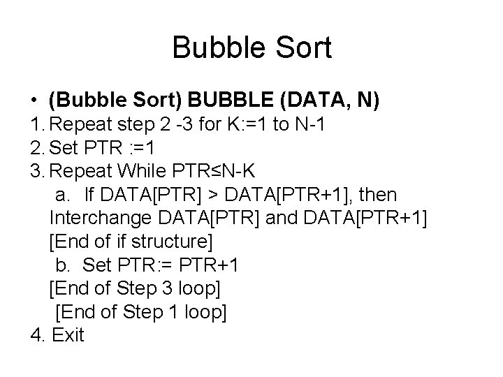
Bubble Sort • (Bubble Sort) BUBBLE (DATA, N) 1. Repeat step 2 -3 for K: =1 to N-1 2. Set PTR : =1 3. Repeat While PTR≤N-K a. If DATA[PTR] > DATA[PTR+1], then Interchange DATA[PTR] and DATA[PTR+1] [End of if structure] b. Set PTR: = PTR+1 [End of Step 3 loop] [End of Step 1 loop] 4. Exit

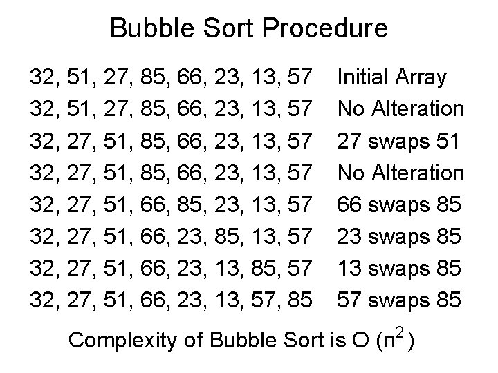
Bubble Sort Procedure 32, 51, 27, 85, 66, 23, 13, 57 32, 27, 51, 66, 85, 23, 13, 57 32, 27, 51, 66, 23, 85, 13, 57 32, 27, 51, 66, 23, 13, 85, 57 32, 27, 51, 66, 23, 13, 57, 85 Initial Array No Alteration 27 swaps 51 No Alteration 66 swaps 85 23 swaps 85 13 swaps 85 57 swaps 85 Complexity of Bubble Sort is O (n 2 )

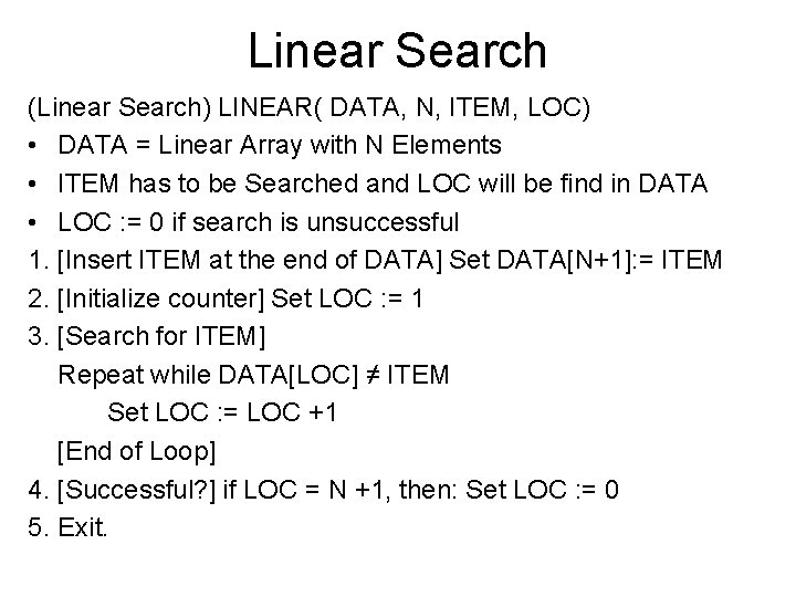
Linear Search (Linear Search) LINEAR( DATA, N, ITEM, LOC) • DATA = Linear Array with N Elements • ITEM has to be Searched and LOC will be find in DATA • LOC : = 0 if search is unsuccessful 1. [Insert ITEM at the end of DATA] Set DATA[N+1]: = ITEM 2. [Initialize counter] Set LOC : = 1 3. [Search for ITEM] Repeat while DATA[LOC] ≠ ITEM Set LOC : = LOC +1 [End of Loop] 4. [Successful? ] if LOC = N +1, then: Set LOC : = 0 5. Exit.

Binary Search (Binary Search) BINARY (DATA, LB, UB, ITEM, LOC) • DATA Sorted Array with Lower Bound LB and Upper Bound UB. LOC of ITEM will be searched by the algorithm or set the LOC = NULL 1. [Initialize segment variables] Set BEG : = LB, END : = UB and MID = INT ((BEG+END)/2) 2. Repeat Step 3 and 4 while BEG <= END and DATA[MID] ≠ ITEM 3. If ITEM < DATA [MID] , then: Set END : = MID – 1 Else Set BEG : = MID +1 [End of If Structure] 4. Set MID : = INT ((BEG + END)/2)

Binary Search Cont… 5. If DATA [MID] = ITEM, Then: Set LOC : = MID Else Set LOC : = NULL [End of If Structure] 6. Exit

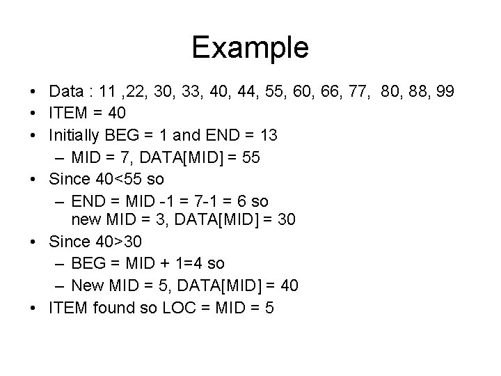
Example • Data : 11 , 22, 30, 33, 40, 44, 55, 60, 66, 77, 80, 88, 99 • ITEM = 40 • Initially BEG = 1 and END = 13 – MID = 7, DATA[MID] = 55 • Since 40<55 so – END = MID -1 = 7 -1 = 6 so new MID = 3, DATA[MID] = 30 • Since 40>30 – BEG = MID + 1=4 so – New MID = 5, DATA[MID] = 40 • ITEM found so LOC = MID = 5

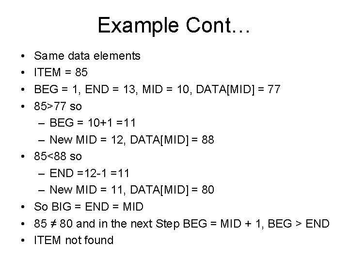
Example Cont… • • Same data elements ITEM = 85 BEG = 1, END = 13, MID = 10, DATA[MID] = 77 85>77 so – BEG = 10+1 =11 – New MID = 12, DATA[MID] = 88 85<88 so – END =12 -1 =11 – New MID = 11, DATA[MID] = 80 So BIG = END = MID 85 ≠ 80 and in the next Step BEG = MID + 1, BEG > END ITEM not found

Complexity in Searching • Linear Search – Time is proportional to n – We call this time complexity O(n) – Both arrays (unsorted) and linked lists • Binary search – Sorted array – Time proportional to log 2 n – Time complexity O(log n) – Only used in arrays

Search with insert and delete • Search and Insert – The ITEM is searched by using any technique appropriate to given DATA – If it is not found ITEM is inserted at the end of DATA • Search and Delete – The ITEM is searched by using any technique appropriate to given DATA – If it is found ITEM is deleted from the DATA – If more than one time ITEM is found than all occurrence are deleted