Some Rules for Expectation Thus you can calculate

Some Rules for Expectation

Thus you can calculate E[Xi] either from the joint distribution of X 1, … , Xn or the marginal distribution of Xi. The Linearity property

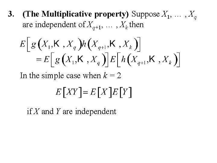
3. (The Multiplicative property) Suppose X 1, … , Xq are independent of Xq+1, … , Xk then In the simple case when k = 2 if X and Y are independent

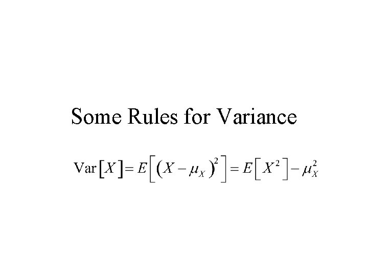
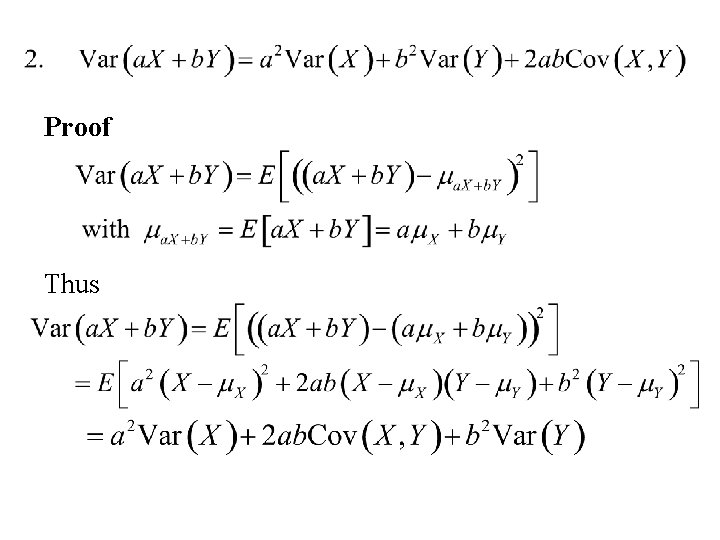
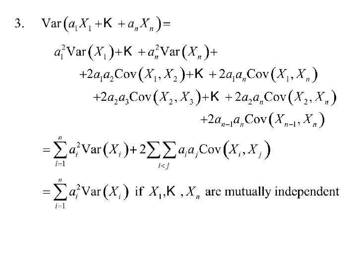
Some Rules for Variance

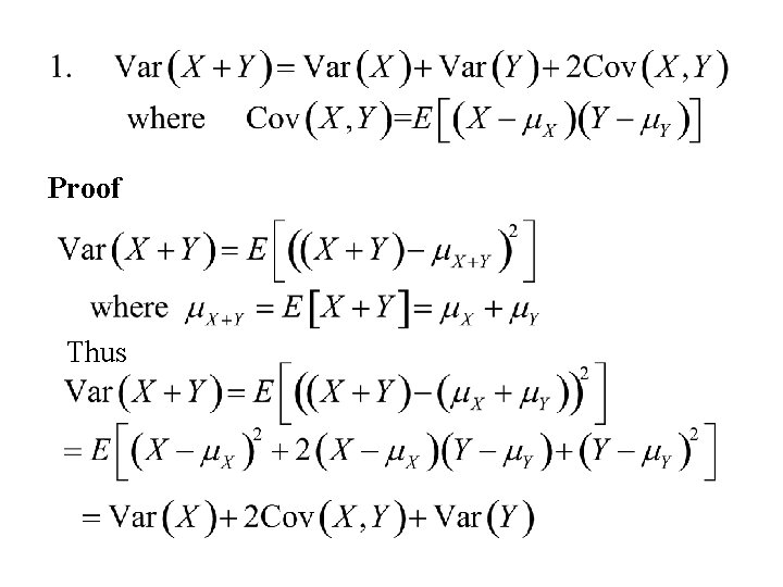
Proof Thus

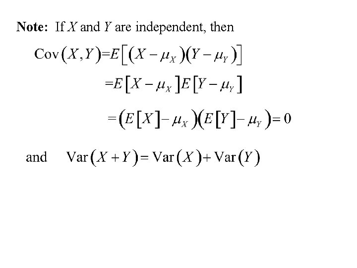
Note: If X and Y are independent, then

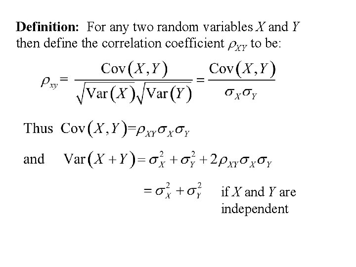
Definition: For any two random variables X and Y then define the correlation coefficient r. XY to be: if X and Y are independent

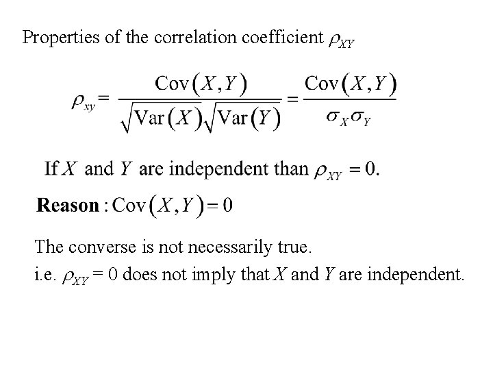
Properties of the correlation coefficient r. XY The converse is not necessarily true. i. e. r. XY = 0 does not imply that X and Y are independent.

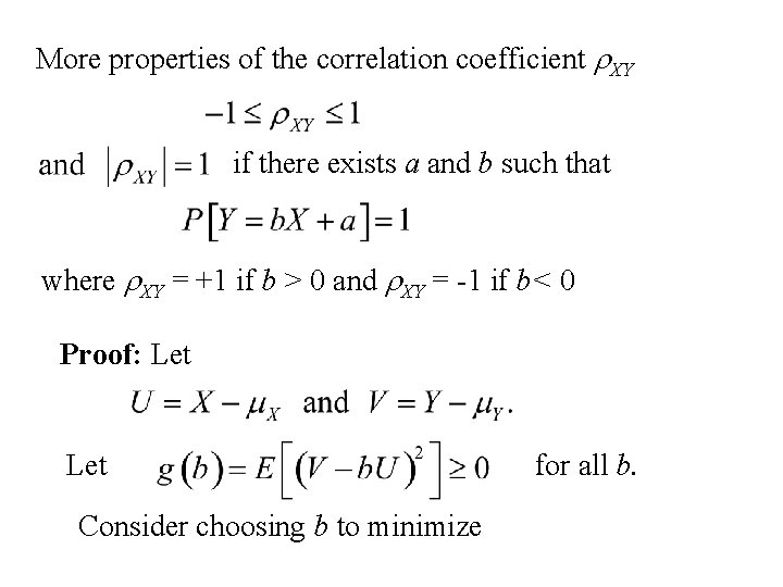
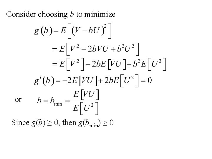
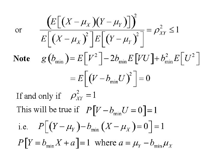
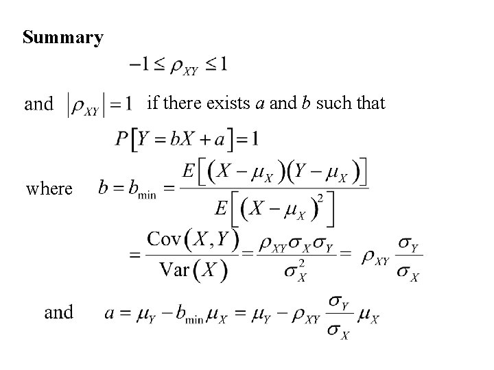
More properties of the correlation coefficient r. XY if there exists a and b such that where r. XY = +1 if b > 0 and r. XY = -1 if b< 0 Proof: Let Consider choosing b to minimize for all b.

Consider choosing b to minimize or Since g(b) ≥ 0, then g(bmin) ≥ 0

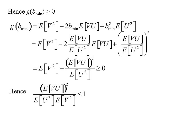
Hence g(bmin) ≥ 0 Hence

or Note If and only if This will be true if i. e.

Summary if there exists a and b such that where

Proof Thus

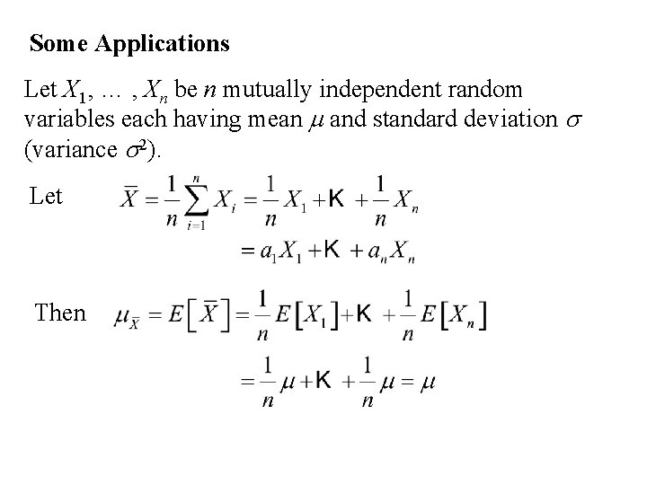
Some Applications Let X 1, … , Xn be n mutually independent random variables each having mean m and standard deviation s (variance s 2). Let Then

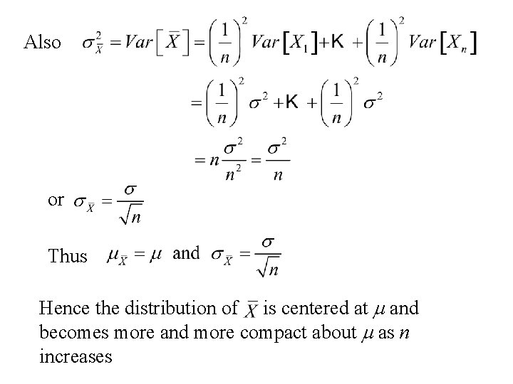
Also or Thus Hence the distribution of is centered at m and becomes more and more compact about m as n increases

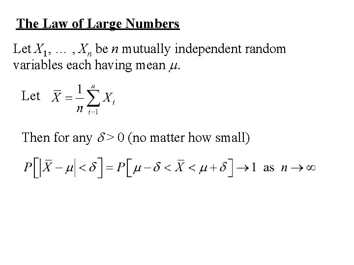
The Law of Large Numbers Let X 1, … , Xn be n mutually independent random variables each having mean m. Let Then for any d > 0 (no matter how small)

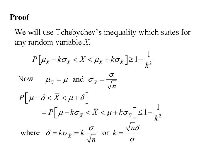
Proof We will use Tchebychev’s inequality which states for any random variable X. Now

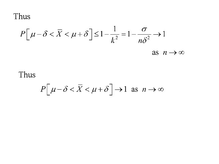
Thus

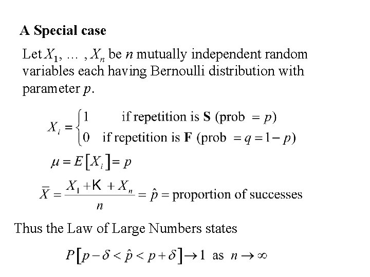
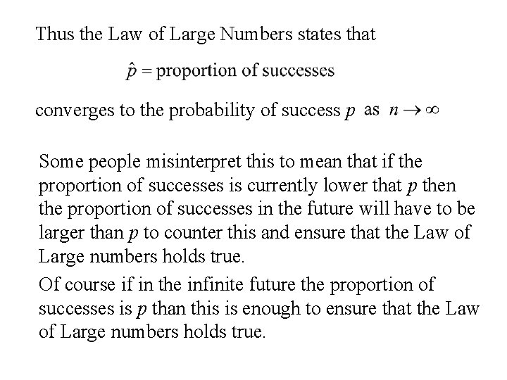
A Special case Let X 1, … , Xn be n mutually independent random variables each having Bernoulli distribution with parameter p. Thus the Law of Large Numbers states

Thus the Law of Large Numbers states that converges to the probability of success p Some people misinterpret this to mean that if the proportion of successes is currently lower that p then the proportion of successes in the future will have to be larger than p to counter this and ensure that the Law of Large numbers holds true. Of course if in the infinite future the proportion of successes is p than this is enough to ensure that the Law of Large numbers holds true.

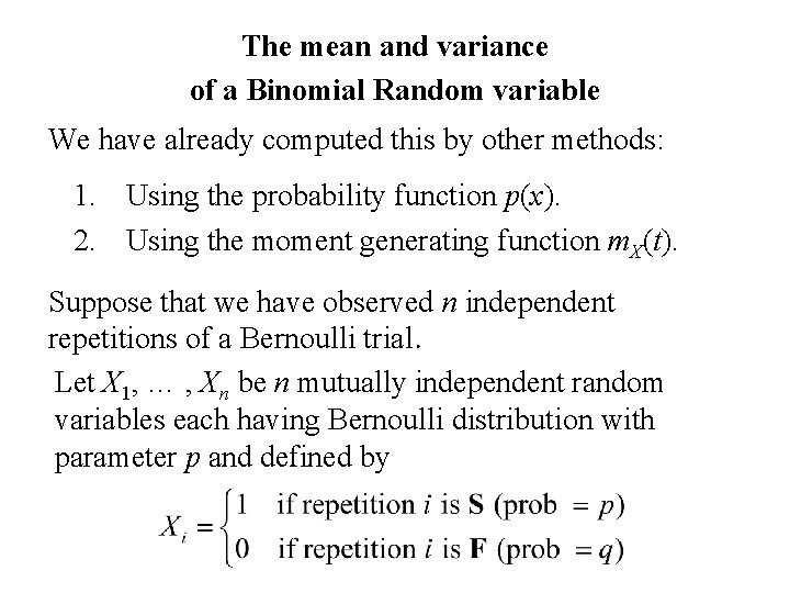
The mean and variance of a Binomial Random variable We have already computed this by other methods: 1. Using the probability function p(x). 2. Using the moment generating function m. X(t). Suppose that we have observed n independent repetitions of a Bernoulli trial. Let X 1, … , Xn be n mutually independent random variables each having Bernoulli distribution with parameter p and defined by

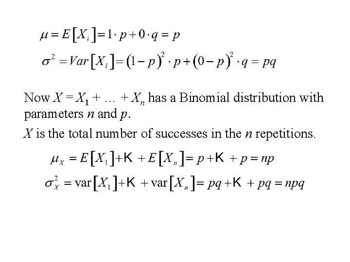
Now X = X 1 + … + Xn has a Binomial distribution with parameters n and p. X is the total number of successes in the n repetitions.

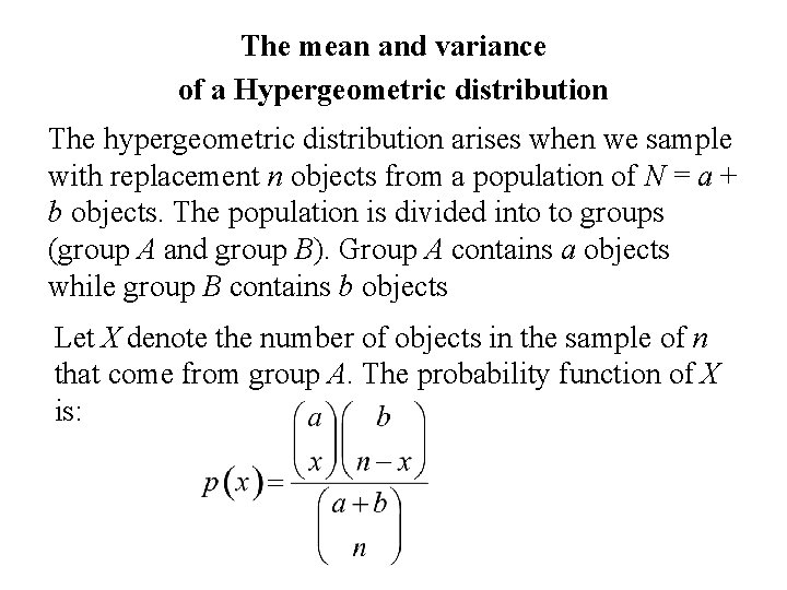
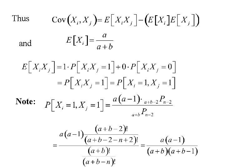
The mean and variance of a Hypergeometric distribution The hypergeometric distribution arises when we sample with replacement n objects from a population of N = a + b objects. The population is divided into to groups (group A and group B). Group A contains a objects while group B contains b objects Let X denote the number of objects in the sample of n that come from group A. The probability function of X is:

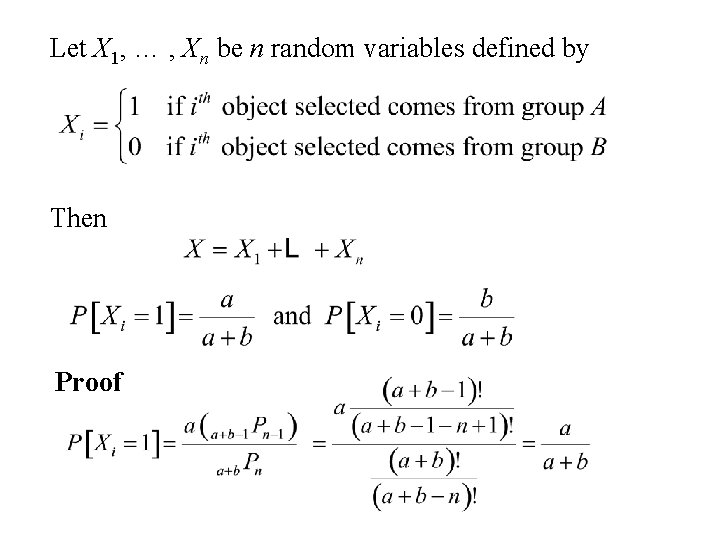
Let X 1, … , Xn be n random variables defined by Then Proof

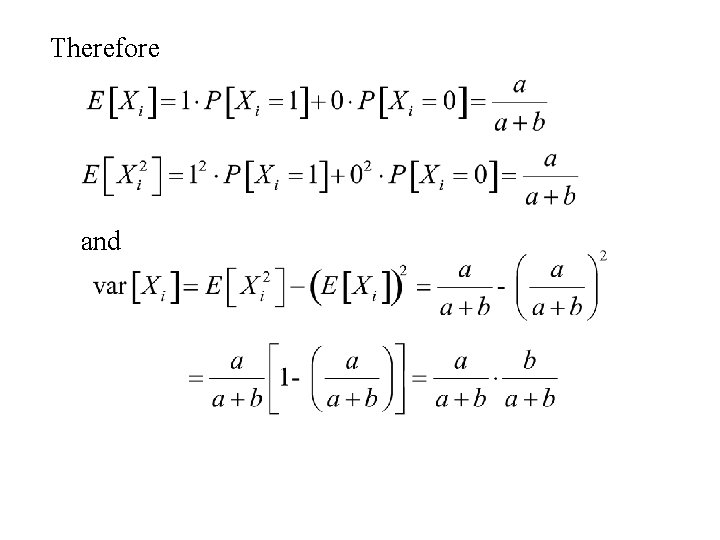
Therefore and

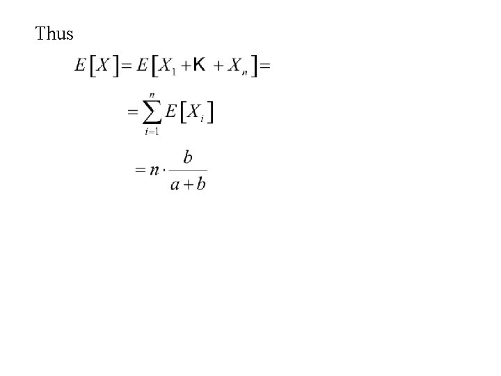
Thus

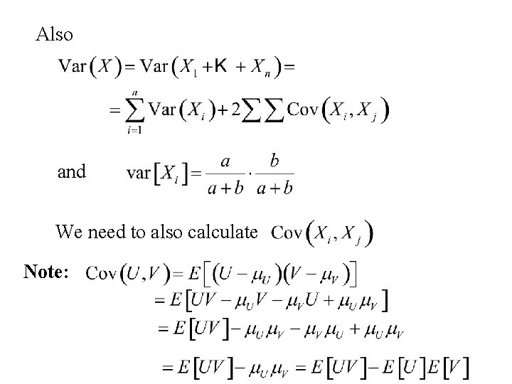
Also and We need to also calculate Note:

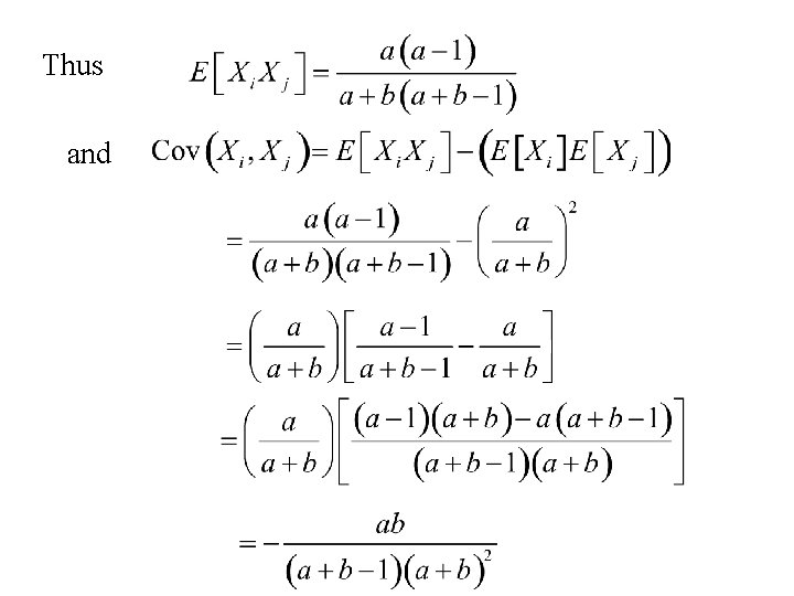
Thus and Note:

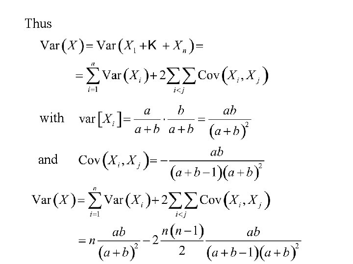
Thus and

Thus with and

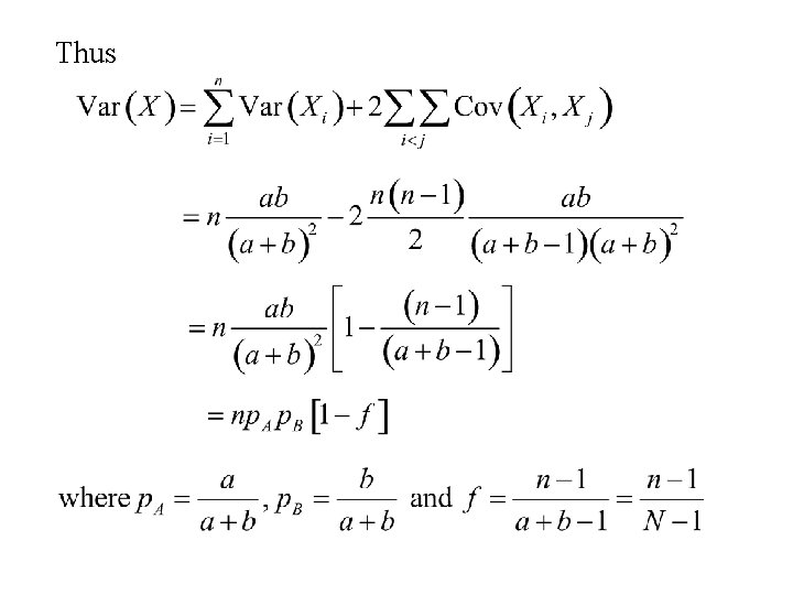
Thus

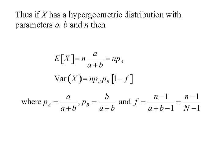
Thus if X has a hypergeometric distribution with parameters a, b and n then

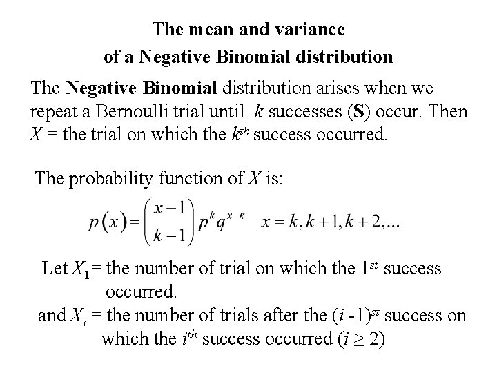
The mean and variance of a Negative Binomial distribution The Negative Binomial distribution arises when we repeat a Bernoulli trial until k successes (S) occur. Then X = the trial on which the kth success occurred. The probability function of X is: Let X 1= the number of trial on which the 1 st success occurred. and Xi = the number of trials after the (i -1)st success on which the ith success occurred (i ≥ 2)

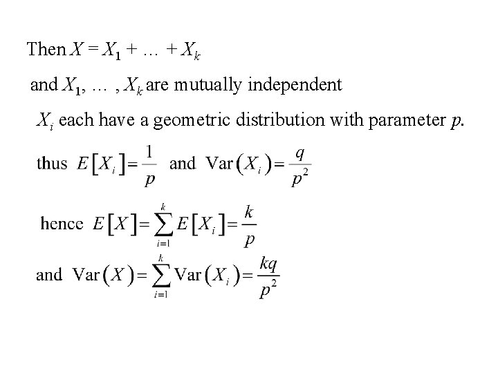
Then X = X 1 + … + Xk and X 1, … , Xk are mutually independent Xi each have a geometric distribution with parameter p.

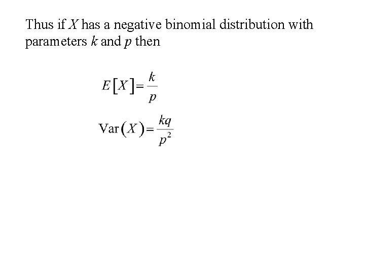
Thus if X has a negative binomial distribution with parameters k and p then