SOME PROBLEMS THAT MIGHT APPEAR IN DATA MULTICOLLINEARITY

SOME PROBLEMS THAT MIGHT APPEAR IN DATA MULTICOLLINEARITY, CONFOUNDING, INTERACTION

MULTICOLLINEARITY HYPOTHETICAL EXAMPLE Case i X 1 i X 2 i Yi 1 2 6 23 2 8 9 83 3 6 8 63 4 10 10 103

HYPTOHETICAL EXAMPLE • Suppose that two statisticians were asked to fit a first order multiple regression model to this data. • The first statistician come up with the following model • The second one used: • Which model is correct?

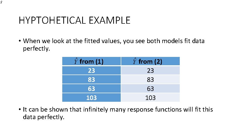
HYPTOHETICAL EXAMPLE • When we look at the fitted values, you see both models fit data perfectly. from (1) 23 83 63 103 from (2) 23 83 63 103 • It can be shown that infinitely many response functions will fit this data perfectly.

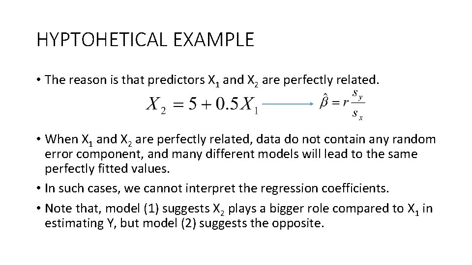
HYPTOHETICAL EXAMPLE • The reason is that predictors X 1 and X 2 are perfectly related. • When X 1 and X 2 are perfectly related, data do not contain any random error component, and many different models will lead to the same perfectly fitted values. • In such cases, we cannot interpret the regression coefficients. • Note that, model (1) suggests X 2 plays a bigger role compared to X 1 in estimating Y, but model (2) suggests the opposite.

MULTICOLLINEARITY • The existence of strong linear relationship between and among the predicted variables in a multiple regression. This is often simply termed collinearity.

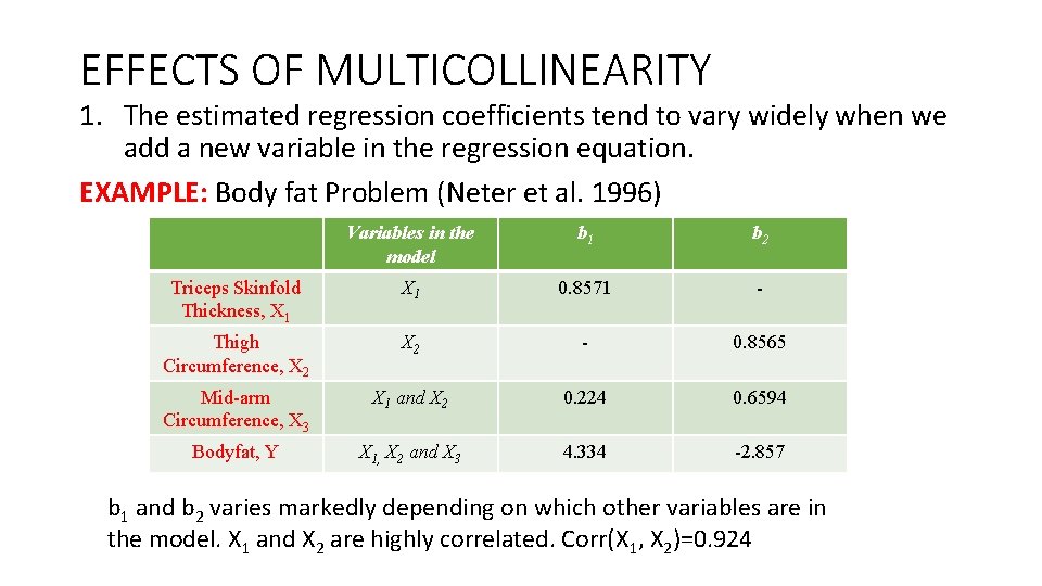
EFFECTS OF MULTICOLLINEARITY 1. The estimated regression coefficients tend to vary widely when we add a new variable in the regression equation. EXAMPLE: Body fat Problem (Neter et al. 1996) Variables in the model b 1 b 2 Triceps Skinfold Thickness, X 1 0. 8571 - Thigh Circumference, X 2 - 0. 8565 Mid-arm Circumference, X 3 X 1 and X 2 0. 224 0. 6594 Bodyfat, Y X 1, X 2 and X 3 4. 334 -2. 857 b 1 and b 2 varies markedly depending on which other variables are in the model. X 1 and X 2 are highly correlated. Corr(X 1, X 2)=0. 924

EFFECTS OF MULTICOLLINEARITY 2. The common interpretation of a regression coefficient is not fully applicable when multicollinearity exists. Normally interpretation of regression coefficients should be “Holding all X’s constant except one, the effect of one unit change of this variable on Y. ” However, when X’s are highly correlated, you cannot really keep one constant and other changing.

EFFECTS OF MULTICOLLINEARITY 3. Estimated regression coefficients b 1 and b 2 changing significantly and become imprecise as more X’s are added to the model when X’s are highly correlated. EXAMPLE: Variables in the s(b 1) s(b 2) model X 1 0. 128 - X 2 - 0. 1100 X 1 and X 2 0. 3034 0. 2912 X 1, X 2 and X 3 3. 016 2. 582 Inflated variability due to multicollinearity

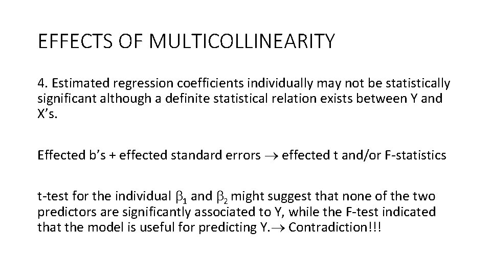
EFFECTS OF MULTICOLLINEARITY 4. Estimated regression coefficients individually may not be statistically significant although a definite statistical relation exists between Y and X’s. Effected b’s + effected standard errors effected t and/or F-statistics t-test for the individual 1 and 2 might suggest that none of the two predictors are significantly associated to Y, while the F-test indicated that the model is useful for predicting Y. Contradiction!!!

EFFECTS OF MULTICOLLINEARITY NO!!! This has to do with the interpretation of the regression coefficients. 1 is the expected change in Y due to X 1 given X 2 is already in the model. 2 is the expected change in Y due to X 2 given X 1 is already in the model. Since both X 1 and X 2 contribute redundant information about Y, once one of the predictors in the model, the other does not have much more to contribute. This is why F-test indicates that at least one of them is important, but individual tests indicate that the contribution of the predictor given the other one already included, is not really important,

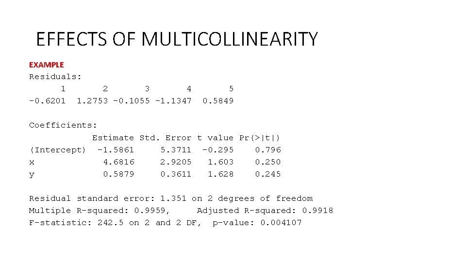
EFFECTS OF MULTICOLLINEARITY EXAMPLE Residuals: 1 2 3 4 5 -0. 6201 1. 2753 -0. 1055 -1. 1347 0. 5849 Coefficients: Estimate Std. Error t value Pr(>|t|) (Intercept) -1. 5861 5. 3711 -0. 295 0. 796 x 4. 6816 2. 9205 1. 603 0. 250 y 0. 5879 0. 3611 1. 628 0. 245 Residual standard error: 1. 351 on 2 degrees of freedom Multiple R-squared: 0. 9959, Adjusted R-squared: 0. 9918 F-statistic: 242. 5 on 2 and 2 DF, p-value: 0. 004107

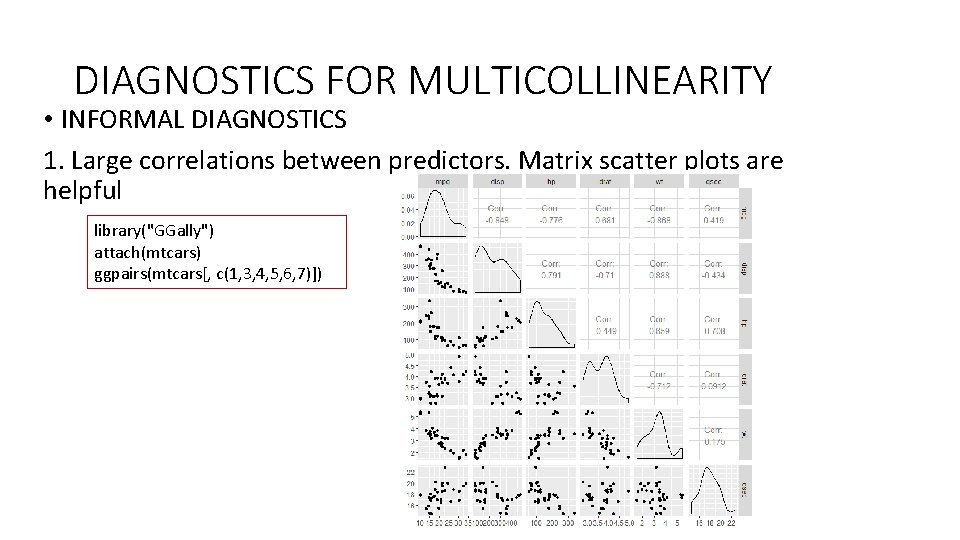
DIAGNOSTICS FOR MULTICOLLINEARITY • INFORMAL DIAGNOSTICS 1. Large correlations between predictors. Matrix scatter plots are helpful library("GGally") attach(mtcars) ggpairs(mtcars[, c(1, 3, 4, 5, 6, 7)])

DIAGNOSTICS FOR MULTICOLLINEARITY • INFORMAL DIAGNOSTICS 2. Indicators of effects of multicollinearity. • Large changes in estimates when more X’s are added or deleted. • t-statistics and F-statistics • Contradictory signs in regression coefficients > summary(model) Call: lm(formula = mpg ~ disp + hp + drat + wt + qsec, data = mtcars) Residuals: Min 1 Q Median 3 Q Max -3. 5404 -1. 6701 -0. 4264 1. 1320 5. 4996 Coefficients: Estimate Std. Error t value Pr(>|t|) (Intercept) 16. 53357 10. 96423 1. 508 0. 14362 disp 0. 00872 0. 01119 0. 779 0. 44281 hp -0. 02060 0. 01528 -1. 348 0. 18936 drat 2. 01578 1. 30946 1. 539 0. 13579 wt -4. 38546 1. 24343 -3. 527 0. 00158 ** qsec 0. 64015 0. 45934 1. 394 0. 17523 --Signif. codes: 0 ‘***’ 0. 001 ‘**’ 0. 01 ‘*’ 0. 05 ‘. ’ 0. 1 ‘ ’ 1 Residual standard error: 2. 558 on 26 degrees of freedom Multiple R-squared: 0. 8489, Adjusted R-squared: 0. 8199 F-statistic: 29. 22 on 5 and 26 DF, p-value: 6. 892 e-10

DIAGNOSTICS FOR MULTICOLLINEARITY •

DIAGNOSTICS FOR MULTICOLLINEARITY •

DIAGNOSTICS FOR MULTICOLLINEARITY # Assume that we are fitting a multiple linear regression on the MTCARS data library(car) fit <- lm(mpg~disp+hp+wt+drat+qsec, data=mtcars) summary(fit) # Evaluate Collinearity vif(fit) # variance inflation factors sum(vif(fit))/4 > 1 > summary(fit) Residuals: Min 1 Q Median 3 Q Max -3. 5404 -1. 6701 -0. 4264 1. 1320 5. 4996 Coefficients: Estimate Std. Error t value Pr(>|t|) (Intercept) 16. 53357 10. 96423 1. 508 0. 14362 disp 0. 00872 0. 01119 0. 779 0. 44281 hp -0. 02060 0. 01528 -1. 348 0. 18936 wt -4. 38546 1. 24343 -3. 527 0. 00158 ** drat 2. 01578 1. 30946 1. 539 0. 13579 qsec 0. 64015 0. 45934 1. 394 0. 17523 --Signif. codes: 0 ‘***’ 0. 001 ‘**’ 0. 01 ‘*’ 0. 05 ‘. ’ 0. 1 ‘ ’ 1 Residual standard error: 2. 558 on 26 degrees of freedom Multiple R-squared: 0. 8489, Adjusted R-squared: 0. 8199 F-statistic: 29. 22 on 5 and 26 DF, p-value: 6. 892 e-10 > vif(fit) # variance inflation factors disp hp wt drat qsec 9. 110869 5. 201833 7. 012686 2. 322343 3. 191939 > sum(vif(fit))/4 > 1 [1] TRUE

REMEDIES FOR MULTICOLLINEARITY •

REMEDIES FOR MULTICOLLINEARITY 2. One or more X’s may be dropped from the model. We can obtain information about the dropped one from the highly correlated one with the response variable. Examine the correlation matrix of Y and all X’s. Drop the one that has low correlation with Y. 3. Principle Component Analysis (PCA) reduces the dimension of uncorrelated components. It may be difficult to attach concrete meanings to the indexes.

REMEDIES FOR MULTICOLLINEARITY • Loss L 2 penalty term

REMEDIES FOR MULTICOLLINEARITY •

REMEDIES FOR MULTICOLLINEARITY > > > x 1 <- rnorm(20) x 2 <- rnorm(20, mean=x 1, sd=. 01) y <- rnorm(20, mean=3+x 1+x 2) fit=lm(y~x 1+x 2) summary(fit) Residuals: Min 1 Q Median 3 Q Max -2. 68064 -0. 97266 0. 08354 0. 97909 1. 76144 Coefficients: Estimate Std. Error t value Pr(>|t|) (Intercept) 3. 2077 0. 3025 10. 603 6. 52 e-09 *** x 1 -8. 8205 34. 7388 -0. 254 0. 803 x 2 11. 1820 34. 6140 0. 323 0. 751 Residual standard error: 1. 345 on 17 degrees of freedom Multiple R-squared: 0. 7209, Adjusted R-squared: 0. 688 F-statistic: 21. 95 on 2 and 17 DF, p-value: 1. 947 e-05 > vif(fit) x 1 x 2 9167. 834 > lm. ridge(y~x 1+x 2, lambda=1) x 1 x 2 3. 202455 1. 160663 1. 178254

REMEDIES FOR MULTICOLLINEARITY 5. LASSO: Least Absolute Shrinkage and Selection Operator The lasso has been introduced by Robert Tibshirani in 1996 and represents another modern approach in regression similar to ridge estimation. He described it in detail in the text book ”The Elements of Statistical Learning” by Hastie, T, Tibshirani, R, Friedman, J (2 nd edition) Springer, available online at https: //web. stanford. edu/~hastie/Papers/ESLII. pdf LASSO methods is a well established method that reduces the variability of the estimates by shrinking the coefficients and at the same time produces interpretable models by shrinking some coefficients to exactly zero.

REMEDIES FOR MULTICOLLINEARITY •

REMEDIES FOR MULTICOLLINEARITY • Loss L 1 penalty term

LIMITATIONS OF LASSO • In small-n-large-p dataset the LASSO selects at most n variables before it saturates. • If there are grouped variables (highly correlated between each other) LASSO tends to select one variable from each group ignoring the others • Elastic Net overcomes LASSO limitations using a combination of LASSO and Ridge Regression methods.

EXAMPLE OF LASSO REGRESSION* • Consider the data from a 1989 study examining the relationship prostatespecific antigen (PSA) and a number of clinical measures in a sample of 97 men who were about to receive a radical prostatectomy (Data from Stamey, T. A. et al. (1989)) • The explanatory variables: o lcavol: Log cancer volume o lweight: Log prostate weight o age o lbph: Log benign prostatic o hyperplasiasvi: Seminal vesicle invasion o lcp: Log capsular penetration o gleason: Gleason score o pgg 45: % Gleason score 4 or 5 * https: //academic. macewan. ca/burok/Stat 378/notes/lasso. pdf

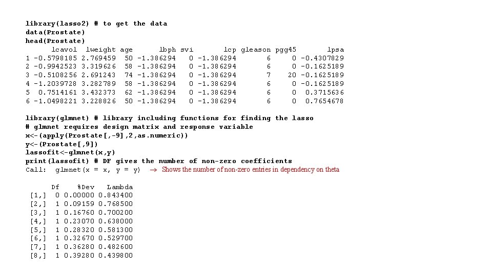
library(lasso 2) # to get the data(Prostate) head(Prostate) lcavol lweight age lbph svi lcp gleason pgg 45 lpsa 1 -0. 5798185 2. 769459 50 -1. 386294 6 0 -0. 4307829 2 -0. 9942523 3. 319626 58 -1. 386294 0 -1. 386294 6 0 -0. 1625189 3 -0. 5108256 2. 691243 74 -1. 386294 0 -1. 386294 7 20 -0. 1625189 4 -1. 2039728 3. 282789 58 -1. 386294 0 -1. 386294 6 0 -0. 1625189 5 0. 7514161 3. 432373 62 -1. 386294 0 -1. 386294 6 0 0. 3715636 6 -1. 0498221 3. 228826 50 -1. 386294 6 0 0. 7654678 library(glmnet) # library including functions for finding the lasso # glmnet requires design matrix and response variable x<-(apply(Prostate[, -9], 2, as. numeric)) y<-(Prostate[, 9]) lassofit<-glmnet(x, y) print(lassofit) # DF gives the number of non-zero coefficients Call: glmnet(x = x, y = y) Shows the number of non-zero entries in dependency on theta Df %Dev Lambda [1, ] 0 0. 00000 0. 843400 [2, ] 1 0. 09159 0. 768500 [3, ] 1 0. 16760 0. 700200 [4, ] 1 0. 23070 0. 638000 [5, ] 1 0. 28320 0. 581300 [6, ] 1 0. 32670 0. 529700 [7, ] 1 0. 36280 0. 482600 [8, ] 1 0. 39280 0. 439800

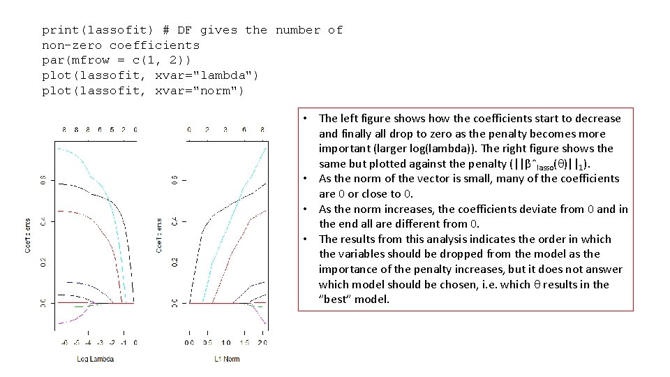
print(lassofit) # DF gives the number of non-zero coefficients par(mfrow = c(1, 2)) plot(lassofit, xvar="lambda") plot(lassofit, xvar="norm") • The left figure shows how the coefficients start to decrease and finally all drop to zero as the penalty becomes more important (larger log(lambda)). The right figure shows the same but plotted against the penalty (||βˆlasso( )||1). • As the norm of the vector is small, many of the coefficients are 0 or close to 0. • As the norm increases, the coefficients deviate from 0 and in the end all are different from 0. • The results from this analysis indicates the order in which the variables should be dropped from the model as the importance of the penalty increases, but it does not answer which model should be chosen, i. e. which results in the ”best” model.

Choosing the tuning parameter, (in many texts, it is given as ) •

Choosing the tuning parameter, •

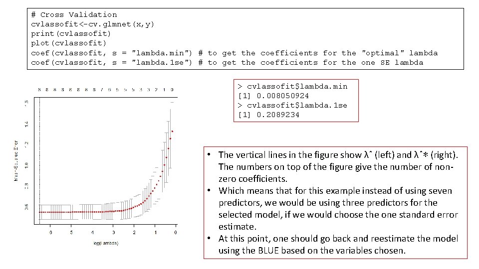
# Cross Validation cvlassofit<-cv. glmnet(x, y) print(cvlassofit) plot(cvlassofit) coef(cvlassofit, s = "lambda. min") # to get the coefficients for the "optimal" lambda coef(cvlassofit, s = "lambda. 1 se") # to get the coefficients for the one SE lambda > cvlassofit$lambda. min [1] 0. 008050924 > cvlassofit$lambda. 1 se [1] 0. 2089234 • The vertical lines in the figure show λˆ (left) and λˆ∗ (right). The numbers on top of the figure give the number of nonzero coefficients. • Which means that for this example instead of using seven predictors, we would be using three predictors for the selected model, if we would choose the one standard error estimate. • At this point, one should go back and reestimate the model using the BLUE based on the variables chosen.

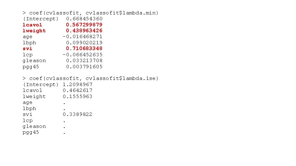
> coef(cvlassofit, cvlassofit$lambda. min) (Intercept) 0. 668454360 lcavol 0. 567299879 lweight 0. 438963426 age -0. 016468271 lbph 0. 099020219 svi 0. 710683348 lcp -0. 066452635 gleason 0. 033213708 pgg 45 0. 003791605 > coef(cvlassofit, cvlassofit$lambda. 1 se) (Intercept) 1. 2098967 lcavol 0. 4642617 lweight 0. 1555963 age . lbph . svi 0. 3389822 lcp . gleason . pgg 45 .

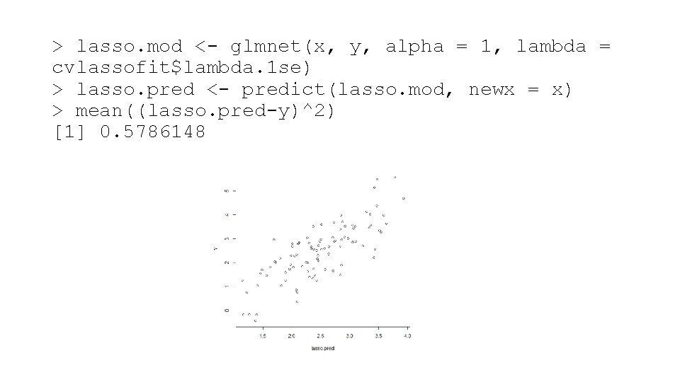
> lasso. mod <- glmnet(x, y, alpha = 1, lambda = cvlassofit$lambda. 1 se) > lasso. pred <- predict(lasso. mod, newx = x) > mean((lasso. pred-y)^2) [1] 0. 5786148

Elastic Net •

Elastic Net • Adding a quadratic part to the penalty, Elastic Net removes the limitation on the selected variables number and stabilize the selection from grouped variables. • The Elastic Net addresses the aforementioned “over-regularization” by balancing between LASSO and ridge penalties. In particular, a hyper-parameter, namely Alpha, would be used to regularize the model such that the model would become a LASSO in case of Alpha = 1 and a ridge in case of Alpha = 0. In practice, Alpha can be tuned easily by the cross-validation. where α is the mixing parameter between ridge (α = 0) and lasso (α = 1).

Variable Selection with Elastic Net pkgs <- list("glmnet", "do. Parallel", "foreach", "p. ROC") lapply(pkgs, require, character. only = T) register. Do. Parallel(cores = 4) df 1 <- read. csv("Downloads/credit_count. txt") df 2 <- df 1[df 1$CARDHLDR == 1, ] set. seed(2017) n <- nrow(df 2) sample <- sample(seq(n), size = n * 0. 5, replace = FALSE) train <- df 2[sample, -1] test <- df 2[-sample, -1] mdl. Y <- as. factor(as. matrix(train["DEFAULT"])) mdl. X <- as. matrix(train[setdiff(colnames(df 1), c("CARDHLDR", "DEFAULT"))]) new. Y <- as. factor(as. matrix(test["DEFAULT"])) new. X <- as. matrix(test[setdiff(colnames(df 1), c("CARDHLDR", "DEFAULT"))])

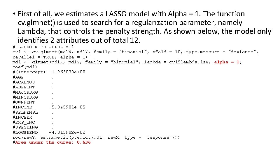
• First of all, we estimates a LASSO model with Alpha = 1. The function cv. glmnet() is used to search for a regularization parameter, namely Lambda, that controls the penalty strength. As shown below, the model only identifies 2 attributes out of total 12. # LASSO WITH ALPHA = 1 cv 1 <- cv. glmnet(mdl. X, mdl. Y, family = "binomial", nfold = 10, type. measure = "deviance", parallel = TRUE, alpha = 1) md 1 <- glmnet(mdl. X, mdl. Y, family = "binomial", lambda = cv 1$lambda. 1 se, alpha = 1) coef(md 1) #(Intercept) -1. 963030 e+00 #AGE . #ACADMOS . #ADEPCNT . #MAJORDRG . #MINORDRG . #OWNRENT . #INCOME -5. 845981 e-05 #SELFEMPL . #INCPER . #EXP_INC . #SPENDING . #LOGSPEND -4. 015902 e-02 roc(new. Y, as. numeric(predict(md 1, new. X, type = "response"))) #Area under the curve: 0. 636

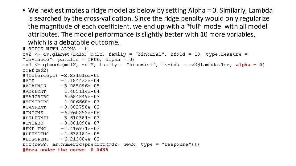
• We next estimates a ridge model as below by setting Alpha = 0. Similarly, Lambda is searched by the cross-validation. Since the ridge penalty would only regularize the magnitude of each coefficient, we end up with a “full” model with all model attributes. The model performance is slightly better with 10 more variables, which is a debatable outcome. # RIDGE WITH ALPHA = 0 cv 2 <- cv. glmnet(mdl. X, mdl. Y, family = "binomial", nfold = 10, type. measure = "deviance", paralle = TRUE, alpha = 0) md 2 <- glmnet(mdl. X, mdl. Y, family = "binomial", lambda = cv 2$lambda. 1 se, alpha = 0) coef(md 2) #(Intercept) -2. 221016 e+00 #AGE -4. 184422 e-04 #ACADMOS -3. 085096 e-05 #ADEPCNT 1. 485114 e-04 #MAJORDRG 6. 684849 e-03 #MINORDRG 1. 006660 e-03 #OWNRENT -9. 082750 e-03 #INCOME -6. 960253 e-06 #SELFEMPL 3. 610381 e-03 #INCPER -3. 881890 e-07 #EXP_INC -1. 416971 e-02 #SPENDING -1. 638184 e-05 #LOGSPEND -6. 213884 e-03 roc(new. Y, as. numeric(predict(md 2, new. X, type = "response"))) #Area under the curve: 0. 6435

• At last, we use the Elastic Net by tuning the value of Alpha through a line search with the parallelism. In this particular case, Alpha = 0. 3 is chosen through the cross-validation. As shown below, 6 variables are used in the model that even performs better than the ridge model with all 12 attributes. # ELASTIC NET WITH 0 < ALPHA < 1 a <- seq(0. 1, 0. 9, 0. 05) search <- foreach(i = a, . combine = rbind) %dopar% { cv <- cv. glmnet(mdl. X, mdl. Y, family = "binomial", nfold = 10, type. measure = "deviance", parallel = TRUE, alpha = i) data. frame(cvm = cv$cvm[cv$lambda == cv$lambda. 1 se], lambda. 1 se = cv$lambda. 1 se, alpha = i) } cv 3 <- search[search$cvm == min(search$cvm), ] md 3 <- glmnet(mdl. X, mdl. Y, family = "binomial", lambda = cv 3$lambda. 1 se, alpha = cv 3$alpha) coef(md 3) #(Intercept) -1. 434700 e+00 #AGE -8. 426525 e-04 #ACADMOS . #ADEPCNT . #MAJORDRG 6. 276924 e-02 #MINORDRG . #OWNRENT -2. 780958 e-02 #INCOME -1. 305118 e-04 #SELFEMPL . #INCPER -2. 085349 e-06 #EXP_INC . #SPENDING . #LOGSPEND -9. 992808 e-02 roc(new. Y, as. numeric(predict(md 3, new. X, type = "response"))) #Area under the curve: 0. 6449