Some more Artificial Intelligence Neural Networks please read

Some more Artificial Intelligence • • Neural Networks please read chapter 19. Genetic Algorithms Genetic Programming Behavior-Based Systems

Background - Neural Networks can be : - Biological models - Artificial models - Desire to produce artificial systems capable of sophisticated computations similar to the human brain.

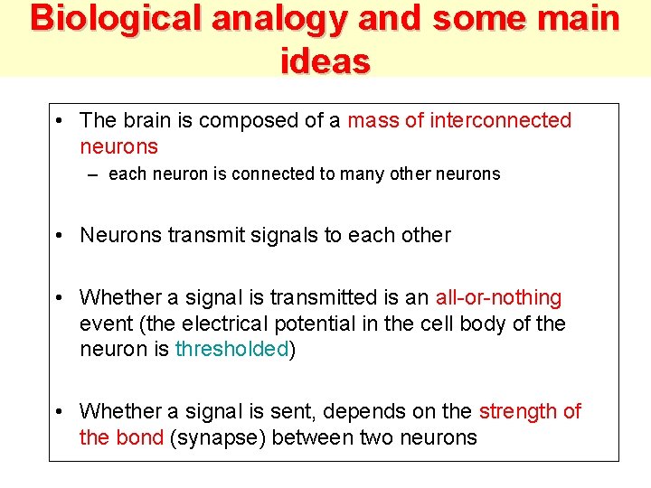
Biological analogy and some main ideas • The brain is composed of a mass of interconnected neurons – each neuron is connected to many other neurons • Neurons transmit signals to each other • Whether a signal is transmitted is an all-or-nothing event (the electrical potential in the cell body of the neuron is thresholded) • Whether a signal is sent, depends on the strength of the bond (synapse) between two neurons

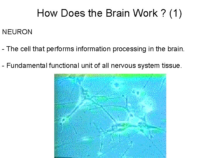
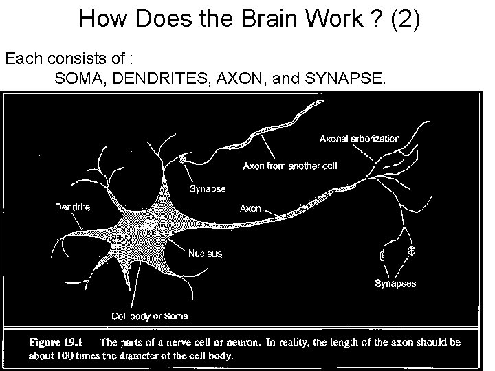
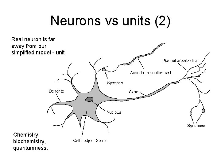
How Does the Brain Work ? (1) NEURON - The cell that performs information processing in the brain. - Fundamental functional unit of all nervous system tissue.

How Does the Brain Work ? (2) Each consists of : SOMA, DENDRITES, AXON, and SYNAPSE.

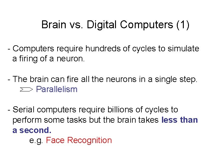
Brain vs. Digital Computers (1) - Computers require hundreds of cycles to simulate a firing of a neuron. - The brain can fire all the neurons in a single step. Parallelism - Serial computers require billions of cycles to perform some tasks but the brain takes less than a second. e. g. Face Recognition

Comparison of Brain and computer

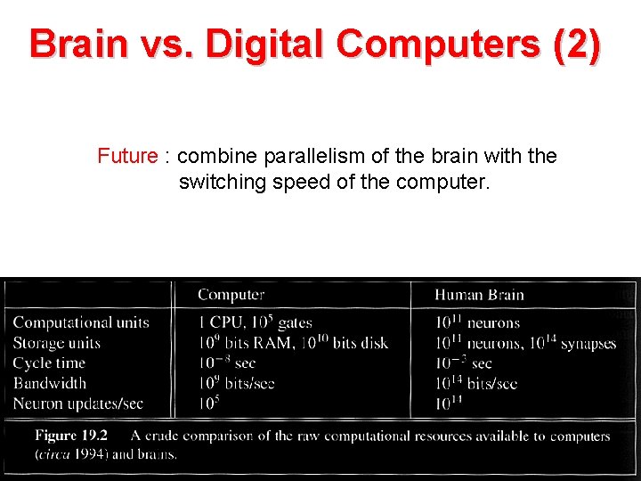
Brain vs. Digital Computers (2) Future : combine parallelism of the brain with the switching speed of the computer.

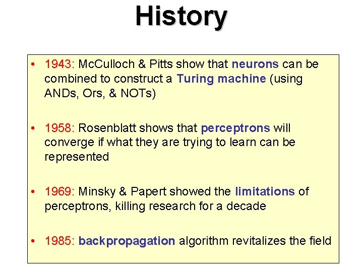
History • 1943: Mc. Culloch & Pitts show that neurons can be combined to construct a Turing machine (using ANDs, Ors, & NOTs) • 1958: Rosenblatt shows that perceptrons will converge if what they are trying to learn can be represented • 1969: Minsky & Papert showed the limitations of perceptrons, killing research for a decade • 1985: backpropagation algorithm revitalizes the field

Definition of Neural Network A Neural Network is a system composed of many simple processing elements operating in parallel which can acquire, store, and utilize experiential knowledge.

What is Artificial Neural Network?

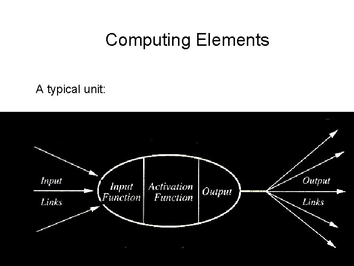
Neurons vs. Units (1) - Each element of NN is a node called unit. - Units are connected by links. - Each link has a numeric weight.

Neurons vs units (2) Real neuron is far away from our simplified model - unit Chemistry, biochemistry, quantumness.

Computing Elements A typical unit:

Planning in building a Neural Network Decisions must be taken on the following: - The number of units to use. - The type of units required. - Connection between the units.

How NN learns a task. Issues to be discussed - Initializing the weights. - Use of a learning algorithm. - Set of training examples. - Encode the examples as inputs. - Convert output into meaningful results.

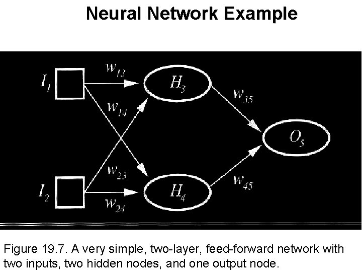
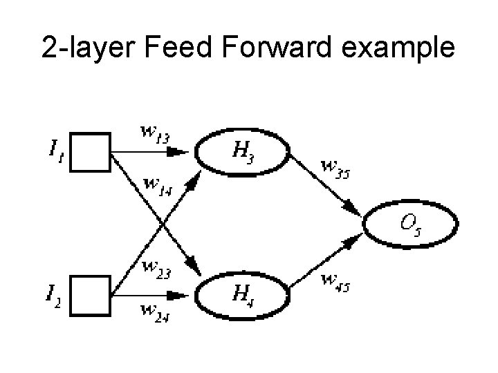
Neural Network Example Figure 19. 7. A very simple, two-layer, feed-forward network with two inputs, two hidden nodes, and one output node.

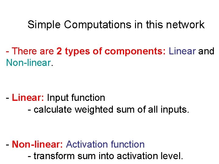
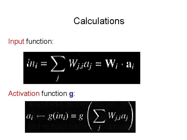
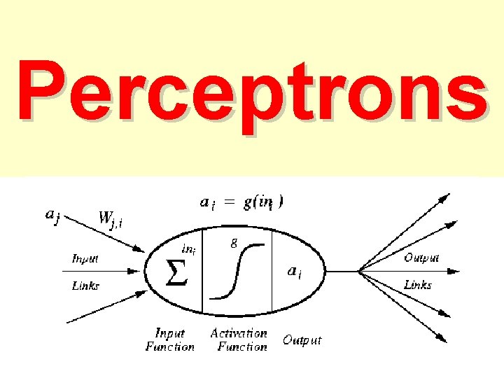
Simple Computations in this network - There are 2 types of components: Linear and Non-linear. - Linear: Input function - calculate weighted sum of all inputs. - Non-linear: Activation function - transform sum into activation level.

Calculations Input function: Activation function g:

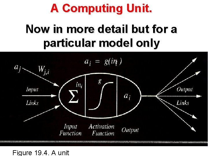
A Computing Unit. Now in more detail but for a particular model only Figure 19. 4. A unit

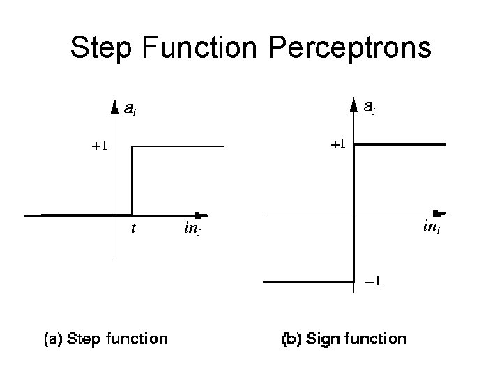
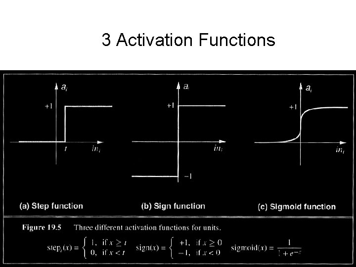
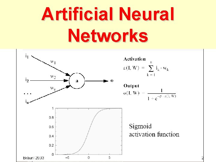
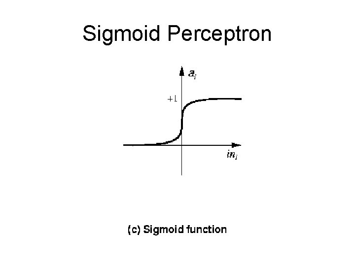
Activation Functions - Use different functions to obtain different models. - 3 most common choices : 1) Step function 2) Sign function 3) Sigmoid function - An output of 1 represents firing of a neuron down the axon.

Step Function Perceptrons

3 Activation Functions

Are current computer a wrong model of thinking? • Humans can’t be doing the sequential analysis we are studying – Neurons are a million times slower than gates – Humans don’t need to be rebooted or debugged when one bit dies.

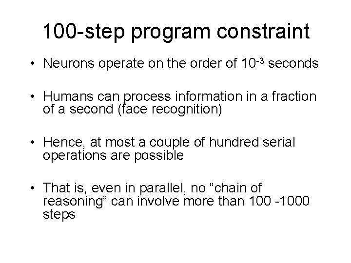
100 -step program constraint • Neurons operate on the order of 10 -3 seconds • Humans can process information in a fraction of a second (face recognition) • Hence, at most a couple of hundred serial operations are possible • That is, even in parallel, no “chain of reasoning” can involve more than 100 -1000 steps

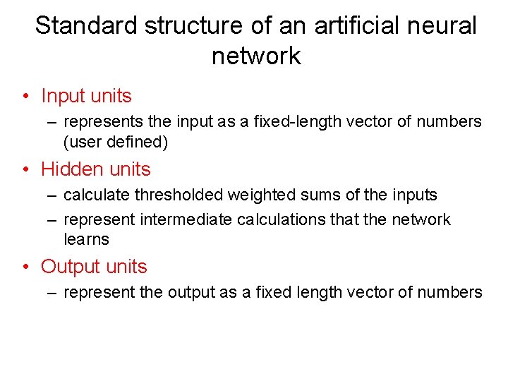
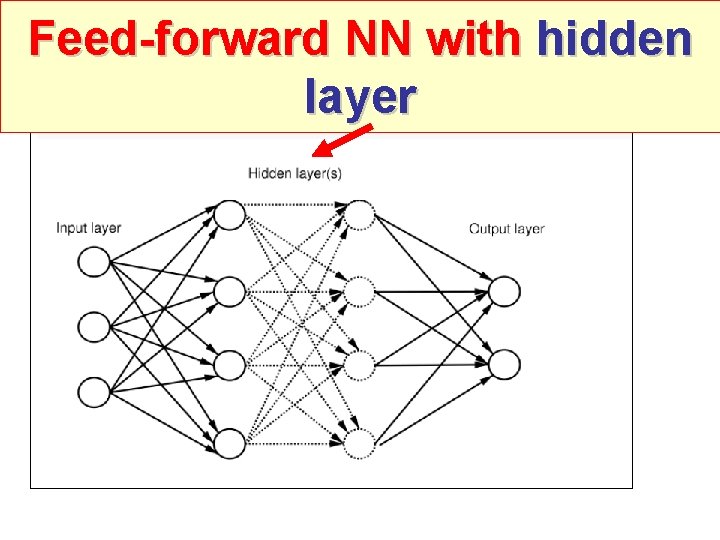
Standard structure of an artificial neural network • Input units – represents the input as a fixed-length vector of numbers (user defined) • Hidden units – calculate thresholded weighted sums of the inputs – represent intermediate calculations that the network learns • Output units – represent the output as a fixed length vector of numbers

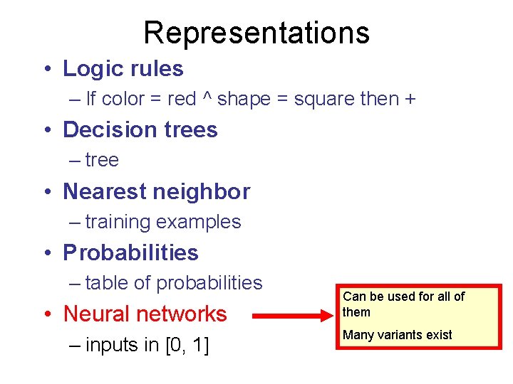
Representations • Logic rules – If color = red ^ shape = square then + • Decision trees – tree • Nearest neighbor – training examples • Probabilities – table of probabilities • Neural networks – inputs in [0, 1] Can be used for all of them Many variants exist

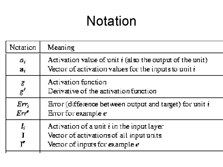
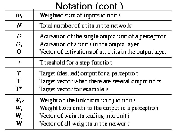
Notations

Notation

Notation (cont. )

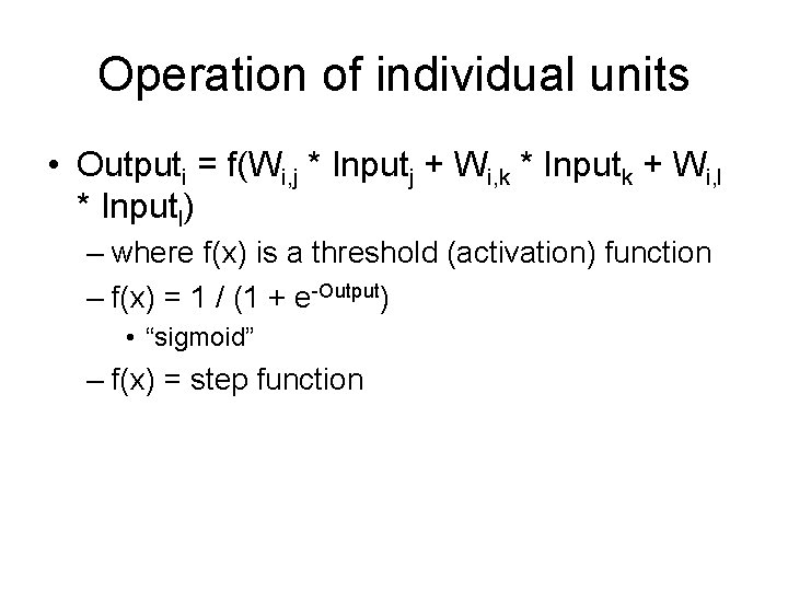
Operation of individual units • Outputi = f(Wi, j * Inputj + Wi, k * Inputk + Wi, l * Inputl) – where f(x) is a threshold (activation) function – f(x) = 1 / (1 + e-Output) • “sigmoid” – f(x) = step function

Artificial Neural Networks

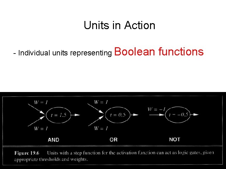
Units in Action - Individual units representing Boolean functions

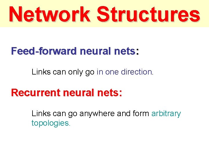
Network Structures Feed-forward neural nets: Links can only go in one direction. Recurrent neural nets: Links can go anywhere and form arbitrary topologies.

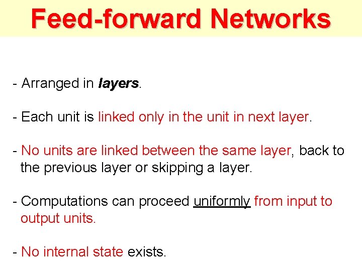
Feed-forward Networks - Arranged in layers - Each unit is linked only in the unit in next layer. - No units are linked between the same layer, back to the previous layer or skipping a layer. - Computations can proceed uniformly from input to output units. - No internal state exists.

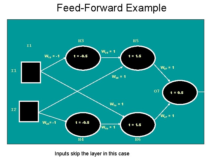
Feed-Forward Example H 3 I 1 W 13 = -1 t = -0. 5 H 5 W 35 = 1 t = 1. 5 W 57 = 1 I 1 W 25 = 1 O 7 t = 0. 5 W 16 = 1 I 2 W 67 = 1 W 24= -1 t = -0. 5 W 46 = 1 t = 1. 5 H 4 Inputs skip the layer in this case H 6

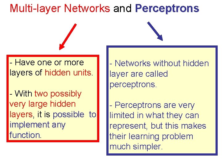
Multi-layer Networks and Perceptrons - Have one or more layers of hidden units. - With two possibly very large hidden layers, it is possible to implement any function - Networks without hidden layer are called perceptrons. - Perceptrons are very limited in what they can represent, but this makes their learning problem much simpler.

Recurrent Network (1) - The brain is not and cannot be a feed-forward network. - Allows activation to be fed back to the previous unit. - Internal state is stored in its activation level. - Can become unstable -Can oscillate.

Recurrent Network (2) - May take long time to compute a stable output. - Learning process is much more difficult. - Can implement more complex designs. - Can model certain systems with internal states.

Perceptrons

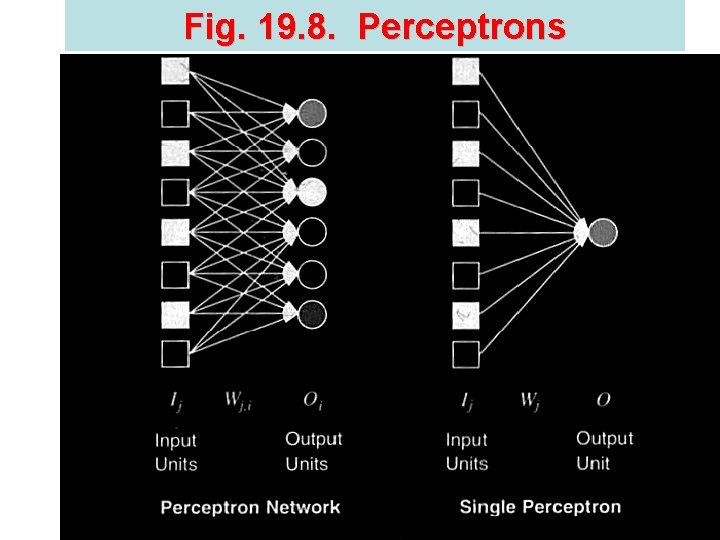
Perceptrons - First studied in the late 1950 s. - Also known as Layered Feed-Forward Networks. - The only efficient learning element at that time was for single-layered networks. - Today, used as a synonym for a single-layer, feed-forward network.

Fig. 19. 8. Perceptrons

Perceptrons

Sigmoid Perceptron

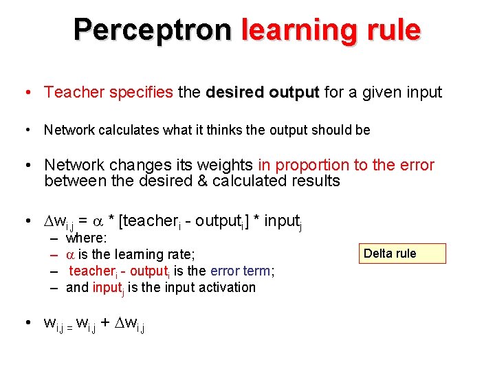
Perceptron learning rule • Teacher specifies the desired output for a given input • Network calculates what it thinks the output should be • Network changes its weights in proportion to the error between the desired & calculated results • wi, j = * [teacheri - outputi] * inputj – – where: is the learning rate; teacheri - outputi is the error term; and inputj is the input activation • wi, j = wi, j + wi, j Delta rule

Adjusting perceptron weights • • wi, j = * [teacheri - outputi] * inputj missi is (teacheri - outputi) • Adjust each wi, j based on inputj and missi • • The above table shows adaptation. Incremental learning.

Node biases • A node’s output is a weighted function of its inputs • What is a bias? • How can we learn the bias value? • Answer: treat them like just another weight

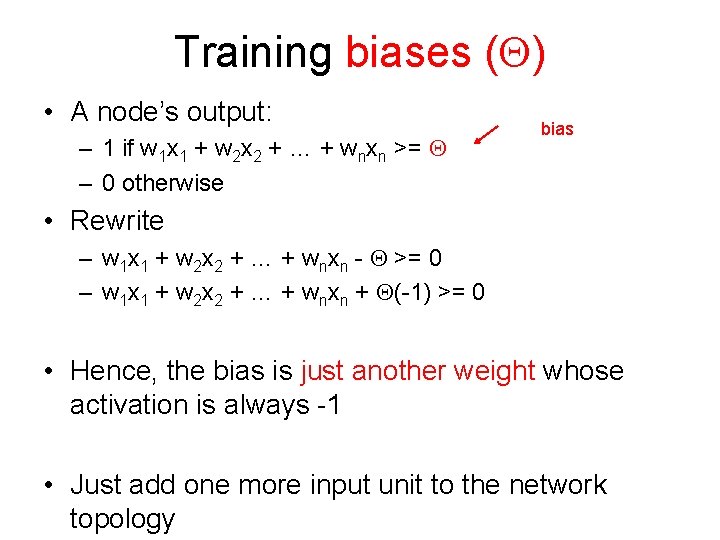
Training biases ( ) • A node’s output: – 1 if w 1 x 1 + w 2 x 2 + … + wnxn >= – 0 otherwise bias • Rewrite – w 1 x 1 + w 2 x 2 + … + wnxn - >= 0 – w 1 x 1 + w 2 x 2 + … + wnxn + (-1) >= 0 • Hence, the bias is just another weight whose activation is always -1 • Just add one more input unit to the network topology

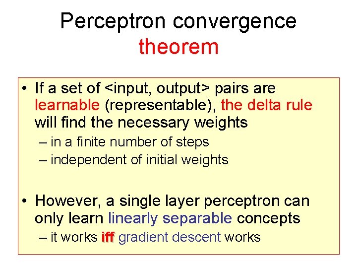
Perceptron convergence theorem • If a set of <input, output> pairs are learnable (representable), the delta rule will find the necessary weights – in a finite number of steps – independent of initial weights • However, a single layer perceptron can only learn linearly separable concepts – it works iff gradient descent works

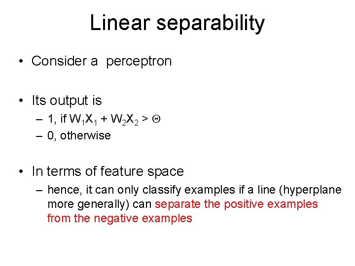
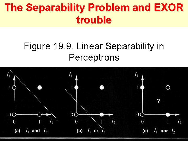
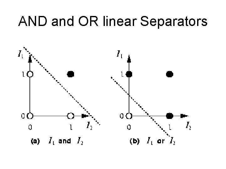
Linear separability • Consider a perceptron • Its output is – 1, if W 1 X 1 + W 2 X 2 > – 0, otherwise • In terms of feature space – hence, it can only classify examples if a line (hyperplane more generally) can separate the positive examples from the negative examples

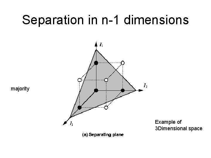
What can Perceptrons Represent ? - Some complex Boolean function can be represented. For example: Majority function - will be covered in this lecture. - Perceptrons are limited in the Boolean functions they can represent.

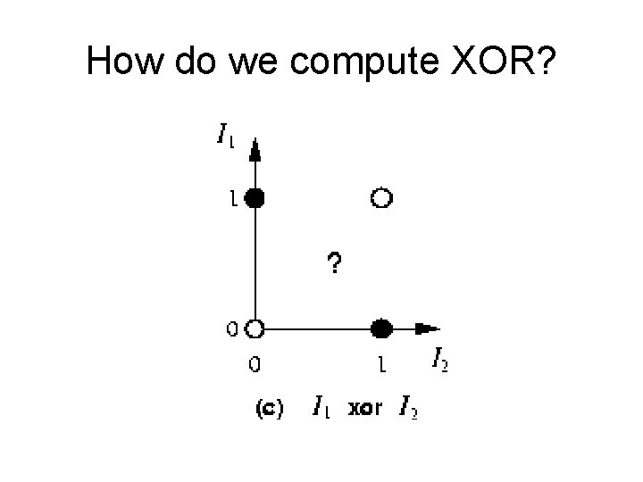
The Separability Problem and EXOR trouble Figure 19. 9. Linear Separability in Perceptrons

AND and OR linear Separators

Separation in n-1 dimensions majority Example of 3 Dimensional space

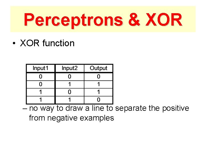
Perceptrons & XOR • XOR function – no way to draw a line to separate the positive from negative examples

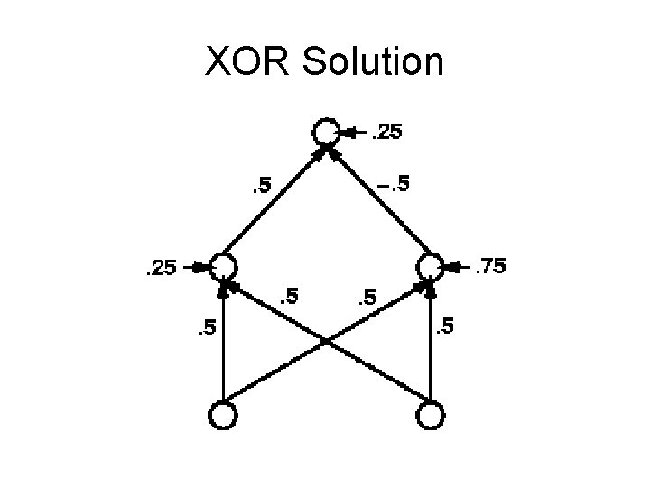
How do we compute XOR?

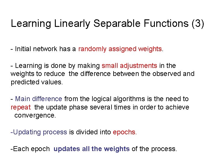
Learning Linearly Separable Functions (1) What can these functions learn ? Bad news: - There are not many linearly separable functions. Good news: - There is a perceptron algorithm that will learn any linearly separable function, given enough training examples.

Learning Linearly Separable Functions (2) Most neural network learning algorithms, including the perceptrons learning method, follow the current-besthypothesis (CBH) scheme.

Learning Linearly Separable Functions (3) - Initial network has a randomly assigned weights. - Learning is done by making small adjustments in the weights to reduce the difference between the observed and predicted values. - Main difference from the logical algorithms is the need to repeat the update phase several times in order to achieve convergence. -Updating process is divided into epochs. -Each epoch updates all the weights of the process.

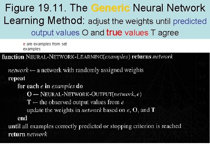
Figure 19. 11. The Generic Neural Network Learning Method: adjust the weights until predicted output values O and true values T agree e are examples from set examples

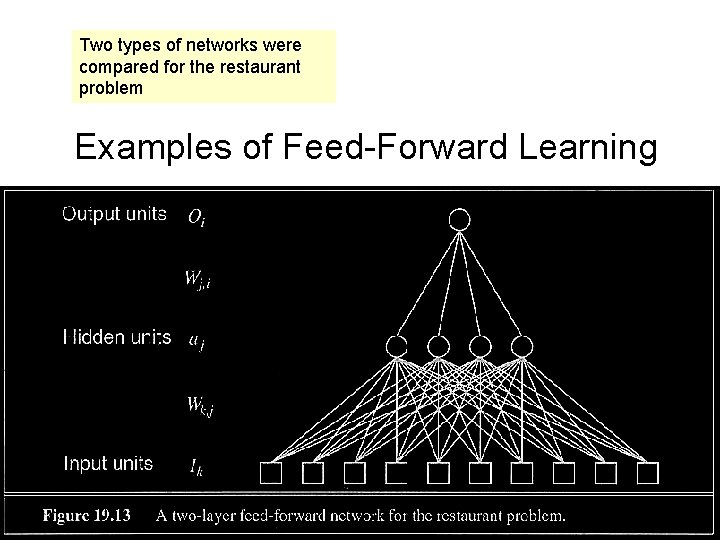
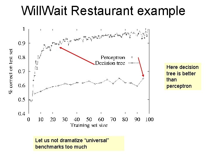
Two types of networks were compared for the restaurant problem Examples of Feed-Forward Learning

Multi-Layer Neural Nets

Feed Forward Networks

2 -layer Feed Forward example

Need for hidden units • If there is one layer of enough hidden units, the input can be recoded (perhaps just memorized; example) • This recoding allows any mapping to be represented • Problem: how can the weights of the hidden units be trained?

XOR Solution

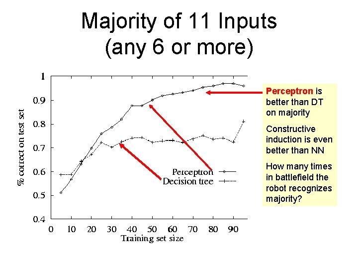
Majority of 11 Inputs (any 6 or more) Perceptron is better than DT on majority Constructive induction is even better than NN How many times in battlefield the robot recognizes majority?

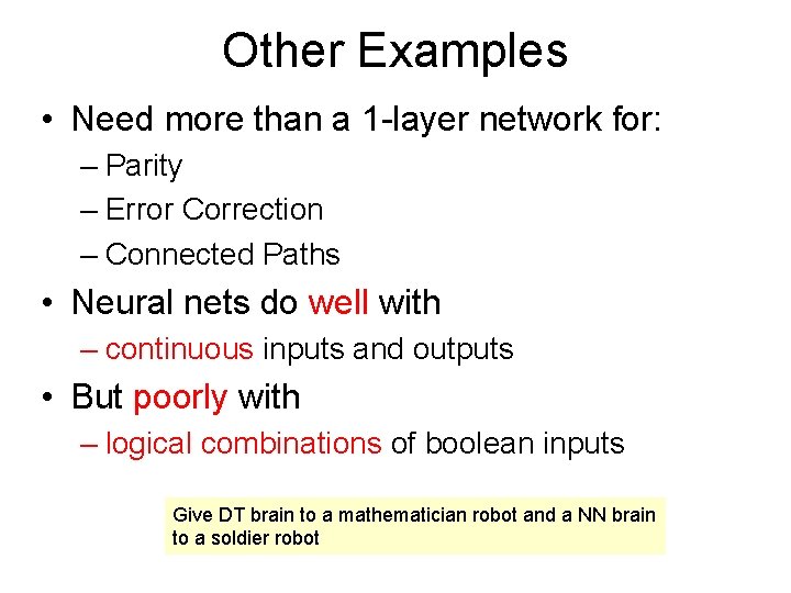
Other Examples • Need more than a 1 -layer network for: – Parity – Error Correction – Connected Paths • Neural nets do well with – continuous inputs and outputs • But poorly with – logical combinations of boolean inputs Give DT brain to a mathematician robot and a NN brain to a soldier robot

Will. Wait Restaurant example Here decision tree is better than perceptron Let us not dramatize “universal” benchmarks too much

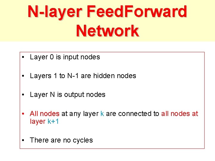
N-layer Feed. Forward Network • Layer 0 is input nodes • Layers 1 to N-1 are hidden nodes • Layer N is output nodes • All nodes at any layer k are connected to all nodes at layer k+1 • There are no cycles

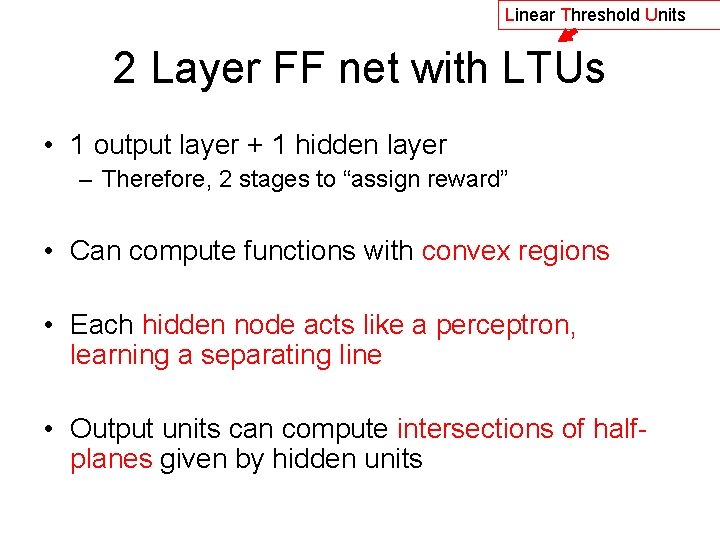
Linear Threshold Units 2 Layer FF net with LTUs • 1 output layer + 1 hidden layer – Therefore, 2 stages to “assign reward” • Can compute functions with convex regions • Each hidden node acts like a perceptron, learning a separating line • Output units can compute intersections of halfplanes given by hidden units

Feed-forward NN with hidden layer

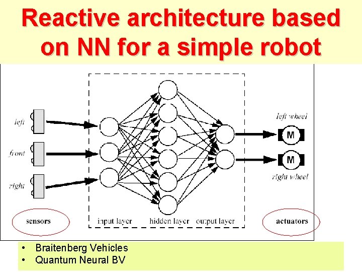
Reactive architecture based on NN for a simple robot • Braitenberg Vehicles • Quantum Neural BV

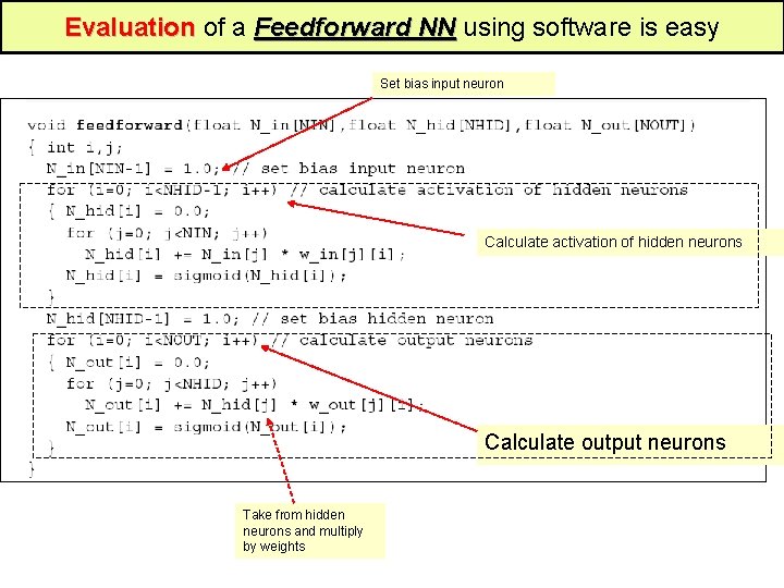
Evaluation of a Feedforward NN using software is easy Set bias input neuron Calculate activation of hidden neurons Calculate output neurons Take from hidden neurons and multiply by weights