Some Computational Science Algorithms Computational science Simulations of

- Slides: 62

Some Computational Science Algorithms

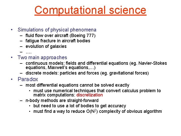
Computational science • Simulations of physical phenomena – – fluid flow over aircraft (Boeing 777) fatigue fracture in aircraft bodies evolution of galaxies …. • Two main approaches – continuous models: fields and differential equations (eg. Navier-Stokes equations, Maxwell’s equations, …) – discrete models: particles and forces (eg. gravitational forces) • Paradox – most differential equations cannot be solved exactly • must use numerical techniques that convert calculus problem to matrix computations: discretization – n-body methods are straight-forward • but need to use a lot of bodies to get accuracy • must find a way to reduce O(N 2) complexity of obvious algorithm

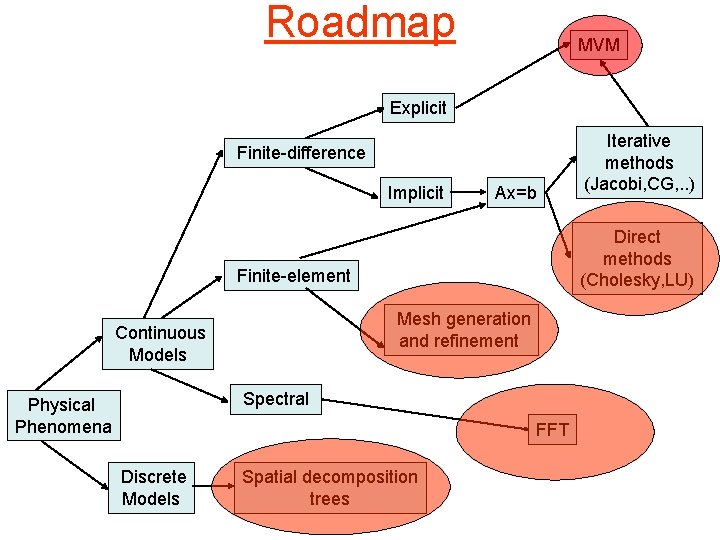
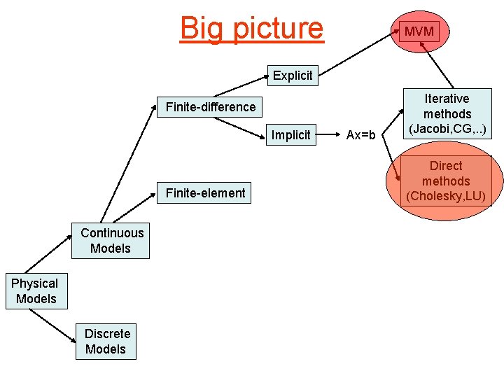
Roadmap MVM Explicit Finite-difference Implicit Ax=b Direct methods (Cholesky, LU) Finite-element Mesh generation and refinement Continuous Models Spectral Physical Phenomena FFT Discrete Models Iterative methods (Jacobi, CG, . . ) Spatial decomposition trees

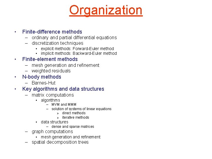
Organization • Finite-difference methods – ordinary and partial differential equations – discretization techniques • explicit methods: Forward-Euler method • implicit methods: Backward-Euler method • Finite-element methods – mesh generation and refinement – weighted residuals • N-body methods – Barnes-Hut • Key algorithms and data structures – matrix computations • algorithms – MVM and MMM – solution of systems of linear equations » direct methods » iterative methods • data structures – dense and sparse matrices – graph computations • mesh generation and refinement – spatial decomposition trees

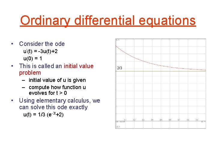
Ordinary differential equations • Consider the ode u‘(t) = -3 u(t)+2 u(0) = 1 • This is called an initial value problem – initial value of u is given – compute how function u evolves for t > 0 • Using elementary calculus, we can solve this ode exactly u(t) = 1/3 (e-3 t+2) 2/3

Problem • For general ode’s, we may not be able to express solution in terms of elementary functions • In most practical situations, we do not need exact solution anyway – enough to compute an approximate solution, provided • we have some idea of how much error was introduced • we can improve the accuracy as needed • General solution: – convert calculus problem into algebra/arithmetic problem • discretization: replace continuous variables with discrete variables • in finite differences, – time will advance in fixed-size steps: t=0, h, 2 h, 3 h, … – differential equation is replaced by difference equation

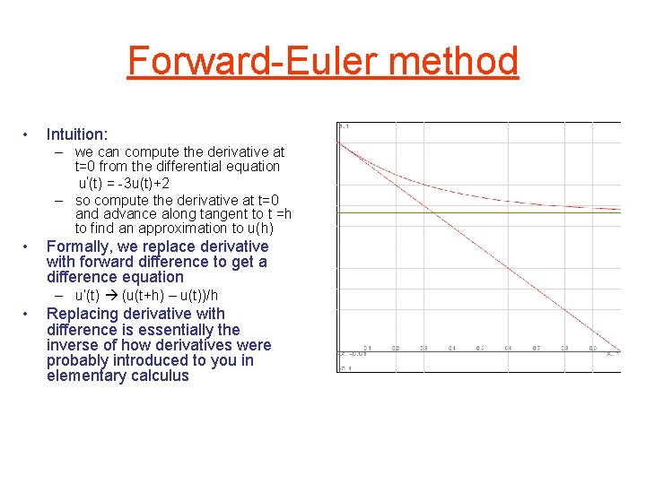
Forward-Euler method • Intuition: – we can compute the derivative at t=0 from the differential equation u‘(t) = -3 u(t)+2 – so compute the derivative at t=0 and advance along tangent to t =h to find an approximation to u(h) • Formally, we replace derivative with forward difference to get a difference equation – u’(t) (u(t+h) – u(t))/h • Replacing derivative with difference is essentially the inverse of how derivatives were probably introduced to you in elementary calculus

Back to ode • Original ode u‘(t) = -3 u(t)+2 • After discretization using Forward-Euler: (uf(t+h) – uf(t))/h = -3 uf(t)+2 • After rearrangement, we get difference equation uf(t+h) = (1 -3 h)uf(t)+2 h • We can now compute values of u: uf(0) = 1 uf(h) = (1 -h) uf(2 h) = (1 -2 h+3 h 2) …. .

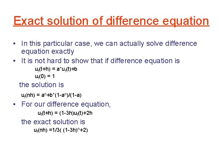
Exact solution of difference equation • In this particular case, we can actually solve difference equation exactly • It is not hard to show that if difference equation is uf(t+h) = a*uf(t)+b uf(0) = 1 the solution is uf(nh) = an+b*(1 -an)/(1 -a) • For our difference equation, uf(t+h) = (1 -3 h)uf(t)+2 h the exact solution is uf(nh) =1/3( (1 -3 h)n+2)

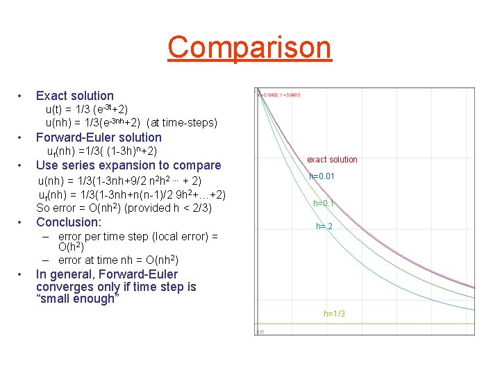
Comparison • Exact solution u(t) = 1/3 (e-3 t+2) u(nh) = 1/3(e-3 nh+2) (at time-steps) • • Forward-Euler solution uf(nh) =1/3( (1 -3 h)n+2) Use series expansion to compare u(nh) = 1/3(1 -3 nh+9/2 n 2 h 2 … + 2) uf(nh) = 1/3(1 -3 nh+n(n-1)/2 9 h 2+…+2) So error = O(nh 2) (provided h < 2/3) • Conclusion: – error per time step (local error) = O(h 2) – error at time nh = O(nh 2) • exact solution h=0. 01 h=0. 1 h=. 2 In general, Forward-Euler converges only if time step is “small enough” h=1/3

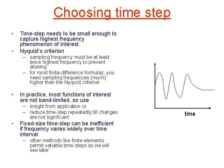
Choosing time step • • Time-step needs to be small enough to capture highest frequency phenomenon of interest Nyquist’s criterion – sampling frequency must be at least twice highest frequency to prevent aliasing – for most finite-difference formulas, you need sampling frequencies (much) higher than the Nyquist criterion • In practice, most functions of interest are not band-limited, so use – insight from application or – reduce time-step repeatedly till changes are not significant • Fixed-size time-step can be inefficient if frequency varies widely over time interval – other methods like finite-elements permit variable time-steps as we will see later time

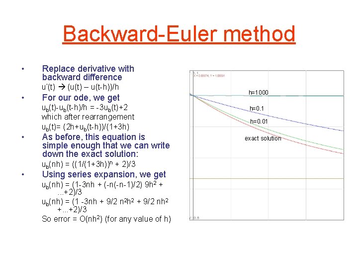
Backward-Euler method • Replace derivative with backward difference u’(t) (u(t) – u(t-h))/h • • • For our ode, we get ub(t)-ub(t-h)/h = -3 ub(t)+2 which after rearrangement ub(t)= (2 h+ub(t-h))/(1+3 h) As before, this equation is simple enough that we can write down the exact solution: ub(nh) = ((1/(1+3 h))n + 2)/3 Using series expansion, we get ub(nh) = (1 -3 nh + (-n(-n-1)/2) 9 h 2 +. . . +2)/3 ub(nh) = (1 -3 nh + 9/2 n 2 h 2 + 9/2 nh 2 +. . . +2)/3 So error = O(nh 2) (for any value of h) h=1000 h=0. 1 h=0. 01 exact solution

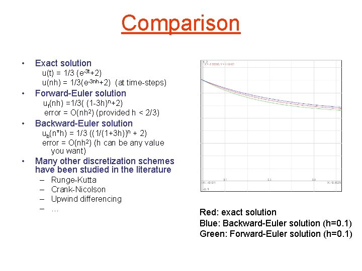
Comparison • Exact solution u(t) = 1/3 (e-3 t+2) u(nh) = 1/3(e-3 nh+2) (at time-steps) • Forward-Euler solution uf(nh) =1/3( (1 -3 h)n+2) error = O(nh 2) (provided h < 2/3) • Backward-Euler solution ub(n*h) = 1/3 ((1/(1+3 h))n + 2) error = O(nh 2) (h can be any value you want) • Many other discretization schemes have been studied in the literature – – Runge-Kutta Crank-Nicolson Upwind differencing … Red: exact solution Blue: Backward-Euler solution (h=0. 1) Green: Forward-Euler solution (h=0. 1)

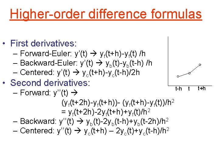
Higher-order difference formulas • First derivatives: – Forward-Euler: y’(t) yf(t+h)-yf(t) /h – Backward-Euler: y’(t) yb(t)-yb(t-h) /h – Centered: y’(t) yc(t+h)-yc(t-h)/2 h • Second derivatives: – Forward: y’’(t) (yf(t+2 h)-yf(t+h))- (yf(t+h)-yf(t))/h 2 = yf(t+2 h)-2 yf(t+h)+yf(t)/h 2 – Backward: y’’(t) yb(t)-2 yb(t-h)+yb(t-2 h)/h 2 – Centered: y’’(t) yc(t+h) – 2 yc(t)+yc(t-h)/h 2 t-h t t+h

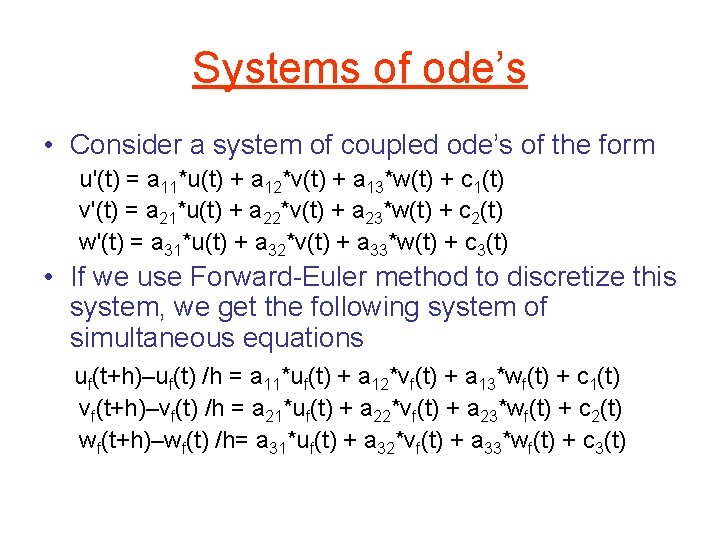
Systems of ode’s • Consider a system of coupled ode’s of the form u'(t) = a 11*u(t) + a 12*v(t) + a 13*w(t) + c 1(t) v'(t) = a 21*u(t) + a 22*v(t) + a 23*w(t) + c 2(t) w'(t) = a 31*u(t) + a 32*v(t) + a 33*w(t) + c 3(t) • If we use Forward-Euler method to discretize this system, we get the following system of simultaneous equations uf(t+h)–uf(t) /h = a 11*uf(t) + a 12*vf(t) + a 13*wf(t) + c 1(t) vf(t+h)–vf(t) /h = a 21*uf(t) + a 22*vf(t) + a 23*wf(t) + c 2(t) wf(t+h)–wf(t) /h= a 31*uf(t) + a 32*vf(t) + a 33*wf(t) + c 3(t)

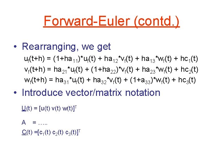
Forward-Euler (contd. ) • Rearranging, we get uf(t+h) = (1+ha 11)*uf(t) + ha 12*vf(t) + ha 13*wf(t) + hc 1(t) vf(t+h) = ha 21*uf(t) + (1+ha 22)*vf(t) + ha 23*wf(t) + hc 2(t) wf(t+h) = ha 31*uf(t) + ha 32*vf(t) + (1+a 33)*wf(t) + hc 3(t) • Introduce vector/matrix notation U(t) = [u(t) v(t) w(t)]T A = …. . C(t) =[c 1(t) c 2(t) c 3(t)]T

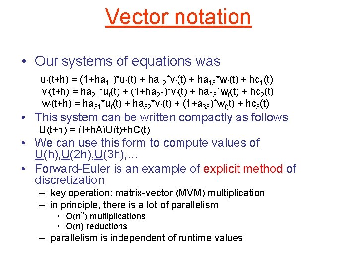
Vector notation • Our systems of equations was uf(t+h) = (1+ha 11)*uf(t) + ha 12*vf(t) + ha 13*wf(t) + hc 1(t) vf(t+h) = ha 21*uf(t) + (1+ha 22)*vf(t) + ha 23*wf(t) + hc 2(t) wf(t+h) = ha 31*uf(t) + ha 32*vf(t) + (1+a 33)*wf(t) + hc 3(t) • This system can be written compactly as follows U(t+h) = (I+h. A)U(t)+h. C(t) • We can use this form to compute values of U(h), U(2 h), U(3 h), … • Forward-Euler is an example of explicit method of discretization – key operation: matrix-vector (MVM) multiplication – in principle, there is a lot of parallelism • O(n 2) multiplications • O(n) reductions – parallelism is independent of runtime values

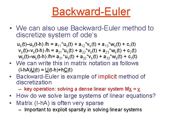
Backward-Euler • We can also use Backward-Euler method to discretize system of ode’s ub(t)–ub(t-h) /h = a 11*ub(t) + a 12*vb(t) + a 13*wb(t) + c 1(t) vb(t)–vb(t-h) /h = a 21*ub(t) + a 22*vb(t) + a 23*wb(t) + c 2(t) wb(t)–wb(t-h) /h= a 31*ub(t) + a 32*vb(t) + a 33*wb(t) + c 3(t) • We can write this in matrix notation as follows (I-h. A)U(t) = U(t-h)+h. C(t) • Backward-Euler is example of implicit method of discretization – key operation: solving a dense linear system Mx = v • How do we solve large systems of linear equations? • Matrix (I-h. A) is often very sparse – Important to exploit sparsity in solving linear systems

Diversion: Solving linear systems

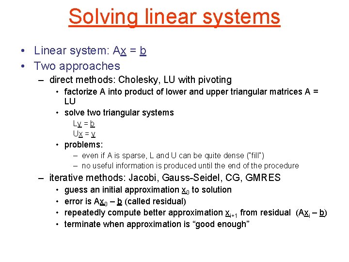
Solving linear systems • Linear system: Ax = b • Two approaches – direct methods: Cholesky, LU with pivoting • factorize A into product of lower and upper triangular matrices A = LU • solve two triangular systems Ly = b Ux = y • problems: – even if A is sparse, L and U can be quite dense (“fill”) – no useful information is produced until the end of the procedure – iterative methods: Jacobi, Gauss-Seidel, CG, GMRES • • guess an initial approximation x 0 to solution error is Ax 0 – b (called residual) repeatedly compute better approximation xi+1 from residual (Axi – b) terminate when approximation is “good enough”

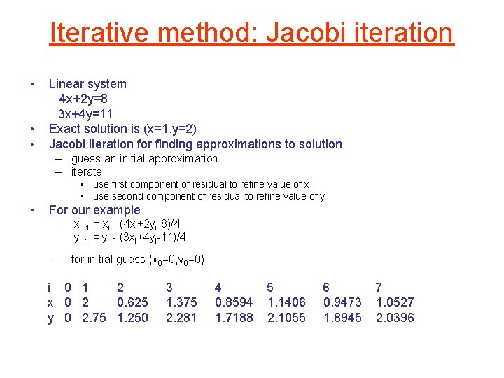
Iterative method: Jacobi iteration • • • Linear system 4 x+2 y=8 3 x+4 y=11 Exact solution is (x=1, y=2) Jacobi iteration for finding approximations to solution – guess an initial approximation – iterate • use first component of residual to refine value of x • use second component of residual to refine value of y • For our example xi+1 = xi - (4 xi+2 yi-8)/4 yi+1 = yi - (3 xi+4 yi-11)/4 – for initial guess (x 0=0, y 0=0) i 0 1 2 x 0 2 0. 625 y 0 2. 75 1. 250 3 1. 375 2. 281 4 0. 8594 1. 7188 5 1. 1406 2. 1055 6 0. 9473 1. 8945 7 1. 0527 2. 0396

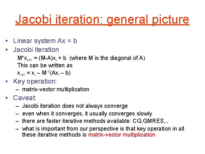
Jacobi iteration: general picture • Linear system Ax = b • Jacobi iteration M*xi+1 = (M-A)xi + b (where M is the diagonal of A) This can be written as xi+1 = xi – M-1(Axi – b) • Key operation: – matrix-vector multiplication • Caveat: – – Jacobi iteration does not always converge even when it converges, it usually converges slowly there are faster iterative methods available: CG, GMRES, . . what is important from our perspective is that key operation in all these iterative methods is matrix-vector multiplication

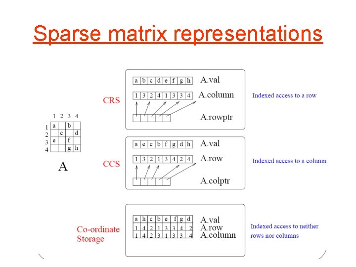
Sparse matrix representations

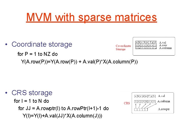
MVM with sparse matrices • Coordinate storage for P = 1 to NZ do Y(A. row(P))=Y(A. row(P)) + A. val(P)*X(A. column(P)) • CRS storage for I = 1 to N do for JJ = A. rowptr(I) to A. row. Ptr(I+1)-1 do Y(I)=Y(I)+A. val(JJ)*X(A. column(J)))

Finite-differences: pde’s

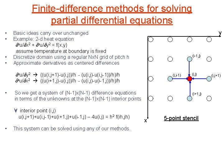
Finite-difference methods for solving partial differential equations • • y Basic ideas carry over unchanged Example: 2 -d heat equation ± 2 u/±x 2 + ± 2 u/±y 2 = f(x, y) assume temperature at boundary is fixed Discretize domain using a regular Nx. N grid of pitch h Approximate derivatives as centered differences (i-1, j) ± 2 u/±y 2 ((u(i, j+1)-u(i, j))/h - (u(i, j)-u(i, j-1))/h)/h ± 2 u/±x 2 ((u(i+1, j)-u(i, j))/h - (u(i, j)-u(i-1, j))/h)/h • So we get a system of (N-1)x(N-1) difference equations in terms of the unknowns at the (N-1)x(N-1) interior points 8 interior point (i, j) u(i, j+1)+u(i, j-1)+u(i+1, j)+u(i-1, j) – 4 u(i, j) = h 2 f(ih, jh) • (i, j-1) This system can be solved using any of our methods. (i, j) (i+1, j) x 5 -point stencil (i, j+1)

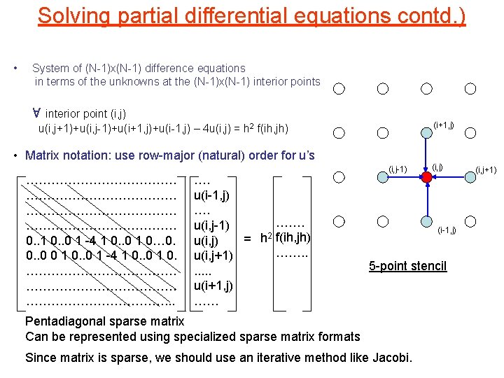
Solving partial differential equations contd. ) • System of (N-1)x(N-1) difference equations in terms of the unknowns at the (N-1)x(N-1) interior points 8 interior point (i, j) u(i, j+1)+u(i, j-1)+u(i+1, j)+u(i-1, j) – 4 u(i, j) = h 2 f(ih, jh) (i+1, j) • Matrix notation: use row-major (natural) order for u’s ……………………………… 0. . 1 0. . 0 1 -4 1 0. . 0 1 0… 0. 0. . 0 0 1 0. . 0 1 -4 1 0. . 0 1 0. ………………………………. . . …. u(i-1, j) …. ……. u(i, j-1) = h 2 f(ih, jh) u(i, j) ……. . u(i, j+1). . . u(i+1, j) …… (i, j-1) (i, j) (i-1, j) 5 -point stencil Pentadiagonal sparse matrix Can be represented using specialized sparse matrix formats Since matrix is sparse, we should use an iterative method like Jacobi. (i, j+1)

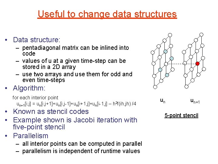
Useful to change data structures • Data structure: – pentadiagonal matrix can be inlined into code – values of u at a given time-step can be stored in a 2 D array – use two arrays and use them for odd and even time-steps • Algorithm: for each interior point un+1[i, j] = un[i, j+1]+un[i, j-1]+un[i+1, j]+un[i-1, j] – h 2 f(ih, jh) /4 • Known as stencil codes • Example shown is Jacobi iteration with five-point stencil • Parallelism – all interior points can be computed in parallel – parallelism is independent of runtime values un un+1 5 -point stencil

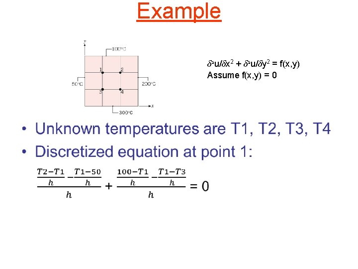
Example ± 2 u/±x 2 + ± 2 u/±y 2 = f(x, y) Assume f(x, y) = 0 •

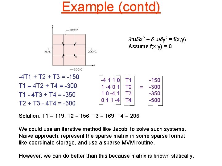
Example (contd) ± 2 u/±x 2 + ± 2 u/±y 2 = f(x, y) Assume f(x, y) = 0 -4 T 1 + T 2 + T 3 = -150 T 1 – 4 T 2 + T 4 = -300 T 1 - 4 T 3 + T 4 = -350 T 2 + T 3 - 4 T 4 = -500 -4 1 1 0 1 -4 0 1 1 0 -4 1 0 1 1 -4 T 1 T 2 T 3 T 4 = -150 -300 -350 -500 Solution: T 1 = 119, T 2 = 156, T 3 = 169, T 4 = 206 We could use an iterative method like Jacobi to solve such systems. Naïve approach: represent the sparse matrix in some sparse format like coordinate storage, and use a sparse MVM routine. However, we can do better than this because matrix is known statically.

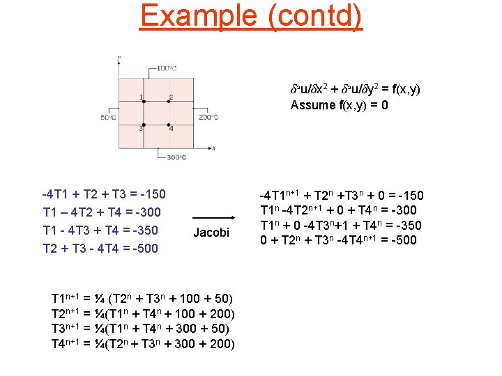
Example (contd) ± 2 u/±x 2 + ± 2 u/±y 2 = f(x, y) Assume f(x, y) = 0 -4 T 1 + T 2 + T 3 = -150 T 1 – 4 T 2 + T 4 = -300 T 1 - 4 T 3 + T 4 = -350 T 2 + T 3 - 4 T 4 = -500 Jacobi T 1 n+1 = ¼ (T 2 n + T 3 n + 100 + 50) T 2 n+1 = ¼(T 1 n + T 4 n + 100 + 200) T 3 n+1 = ¼(T 1 n + T 4 n + 300 + 50) T 4 n+1 = ¼(T 2 n + T 3 n + 300 + 200) -4 T 1 n+1 + T 2 n +T 3 n + 0 = -150 T 1 n -4 T 2 n+1 + 0 + T 4 n = -300 T 1 n + 0 -4 T 3 n+1 + T 4 n = -350 0 + T 2 n + T 3 n -4 T 4 n+1 = -500

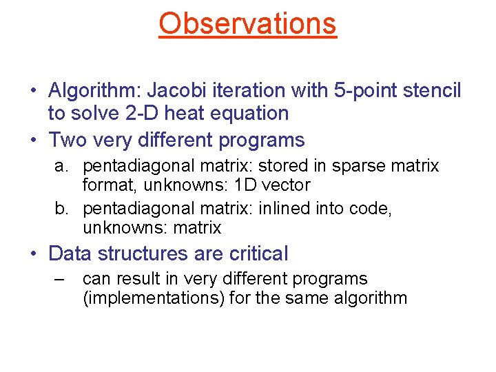
Observations • Algorithm: Jacobi iteration with 5 -point stencil to solve 2 -D heat equation • Two very different programs a. pentadiagonal matrix: stored in sparse matrix format, unknowns: 1 D vector b. pentadiagonal matrix: inlined into code, unknowns: matrix • Data structures are critical – can result in very different programs (implementations) for the same algorithm

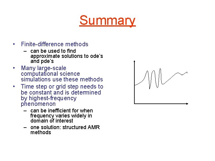
Summary • Finite-difference methods – can be used to find approximate solutions to ode’s and pde’s • Many large-scale computational science simulations use these methods • Time step or grid step needs to be constant and is determined by highest-frequency phenomenon – can be inefficient for when frequency varies widely in domain of interest – one solution: structured AMR methods

Big picture MVM Explicit Finite-difference Implicit Finite-element Continuous Models Physical Models Discrete Models Ax=b Iterative methods (Jacobi, CG, . . ) Direct methods (Cholesky, LU)

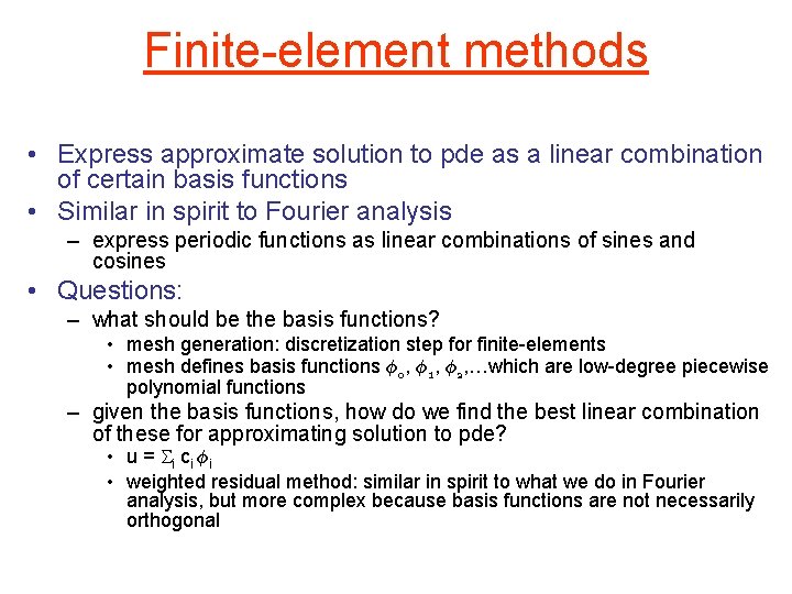
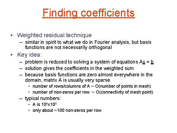
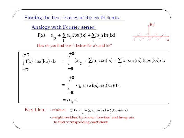
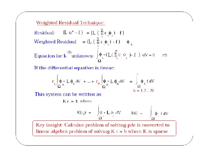
Finite-element methods • Express approximate solution to pde as a linear combination of certain basis functions • Similar in spirit to Fourier analysis – express periodic functions as linear combinations of sines and cosines • Questions: – what should be the basis functions? • mesh generation: discretization step for finite-elements • mesh defines basis functions Á0, Á1, Á2, …which are low-degree piecewise polynomial functions – given the basis functions, how do we find the best linear combination of these for approximating solution to pde? • u = S i c i Ái • weighted residual method: similar in spirit to what we do in Fourier analysis, but more complex because basis functions are not necessarily orthogonal

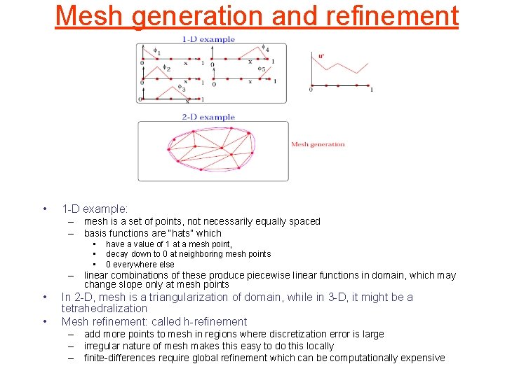
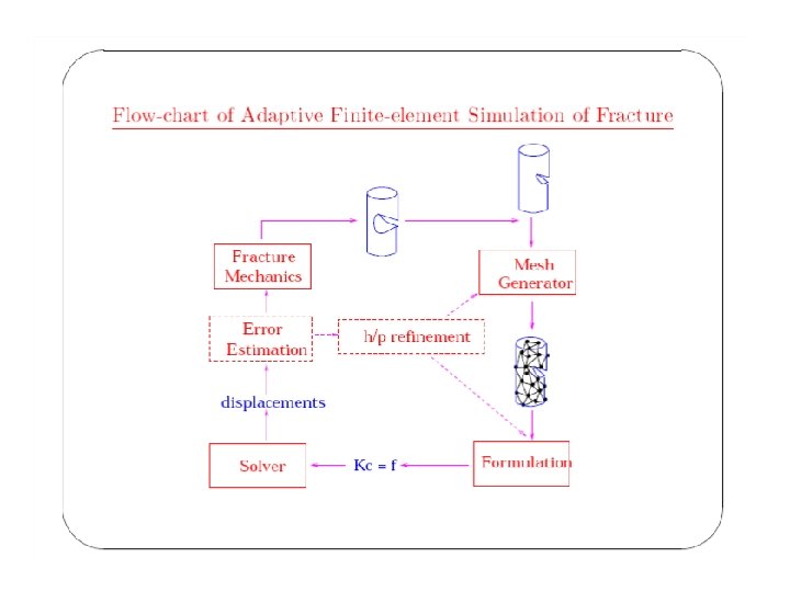
Mesh generation and refinement • 1 -D example: – mesh is a set of points, not necessarily equally spaced – basis functions are “hats” which • • • have a value of 1 at a mesh point, decay down to 0 at neighboring mesh points 0 everywhere else – linear combinations of these produce piecewise linear functions in domain, which may change slope only at mesh points • • In 2 -D, mesh is a triangularization of domain, while in 3 -D, it might be a tetrahedralization Mesh refinement: called h-refinement – add more points to mesh in regions where discretization error is large – irregular nature of mesh makes this easy to do this locally – finite-differences require global refinement which can be computationally expensive

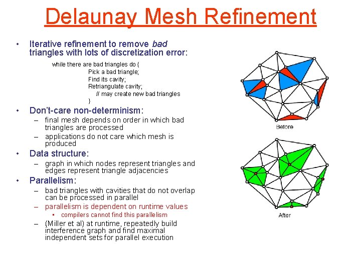
Delaunay Mesh Refinement • Iterative refinement to remove bad triangles with lots of discretization error: while there are bad triangles do { Pick a bad triangle; Find its cavity; Retriangulate cavity; // may create new bad triangles } • Don’t-care non-determinism: – final mesh depends on order in which bad triangles are processed – applications do not care which mesh is produced • Data structure: – graph in which nodes represent triangles and edges represent triangle adjacencies • Parallelism: – bad triangles with cavities that do not overlap can be processed in parallel – parallelism is dependent on runtime values • compilers cannot find this parallelism – (Miller et al) at runtime, repeatedly build interference graph and find maximal independent sets for parallel execution

Finding coefficients • Weighted residual technique – similar in spirit to what we do in Fourier analysis, but basis functions are not necessarily orthogonal • Key idea: – problem is reduced to solving a system of equations Ax = b – solution gives the coefficients in the weighted sum – because basis functions are zero almost everywhere in the domain, matrix A is usually very sparse • number of rows/columns of A ~ O(number of points in mesh) • number of non-zeros per row ~ O(connectivity of mesh point) – typical numbers: • A is 106 x 106 • only about ~100 non-zeros per row


Barnes Hut N-body Simulation

Introduction • Physical system simulation (time evolution) – System consists of bodies – “n” is the number of bodies – Bodies interact via pair-wise forces • Many systems can be modeled in these terms – Galaxy clusters (gravitational force) – Particles (electric force, magnetic force) Barnes Hut N-body Simulation 43

Barnes Hut Idea • Precise force calculation – Requires O(n 2) operations (O(n 2) body pairs) • Barnes and Hut (1986) – Algorithm to approximately compute forces • Bodies’ initial position & velocity are also approximate – Requires only O(n log n) operations – Idea is to “combine” far away bodies – Error should be small because force 1/r 2 Barnes Hut N-body Simulation 44

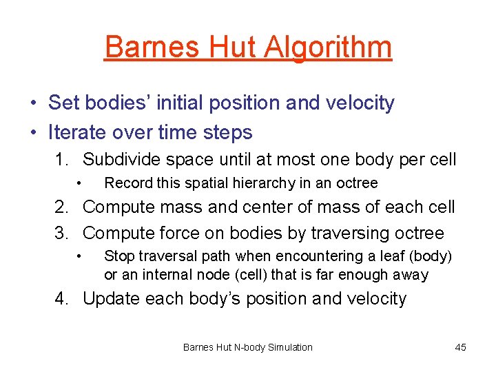
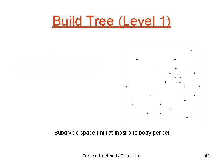
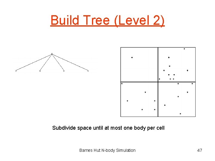
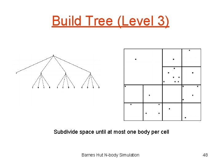
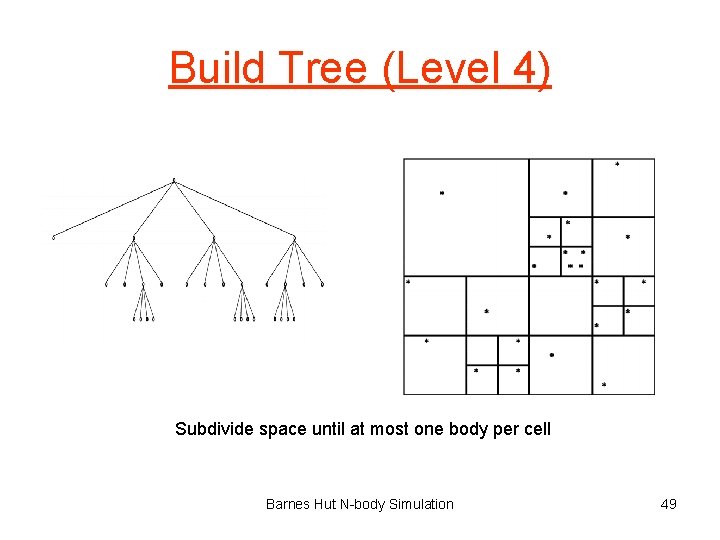
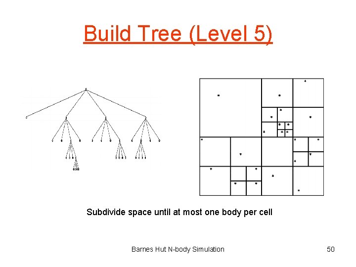
Barnes Hut Algorithm • Set bodies’ initial position and velocity • Iterate over time steps 1. Subdivide space until at most one body per cell • Record this spatial hierarchy in an octree 2. Compute mass and center of mass of each cell 3. Compute force on bodies by traversing octree • Stop traversal path when encountering a leaf (body) or an internal node (cell) that is far enough away 4. Update each body’s position and velocity Barnes Hut N-body Simulation 45

Build Tree (Level 1) Subdivide space until at most one body per cell Barnes Hut N-body Simulation 46

Build Tree (Level 2) Subdivide space until at most one body per cell Barnes Hut N-body Simulation 47

Build Tree (Level 3) Subdivide space until at most one body per cell Barnes Hut N-body Simulation 48

Build Tree (Level 4) Subdivide space until at most one body per cell Barnes Hut N-body Simulation 49

Build Tree (Level 5) Subdivide space until at most one body per cell Barnes Hut N-body Simulation 50

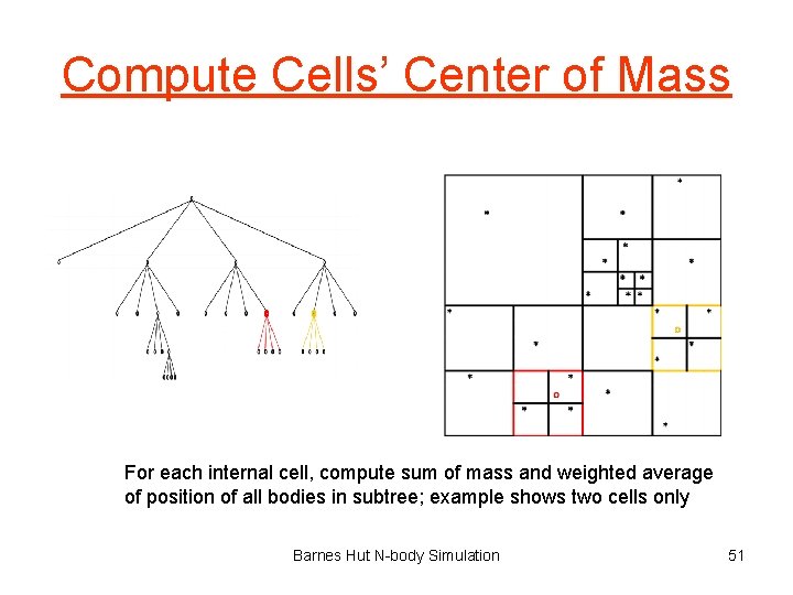
Compute Cells’ Center of Mass For each internal cell, compute sum of mass and weighted average of position of all bodies in subtree; example shows two cells only Barnes Hut N-body Simulation 51

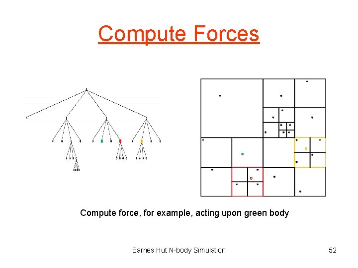
Compute Forces Compute force, for example, acting upon green body Barnes Hut N-body Simulation 52

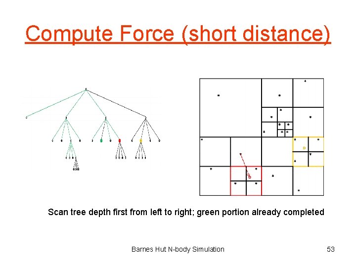
Compute Force (short distance) Scan tree depth first from left to right; green portion already completed Barnes Hut N-body Simulation 53

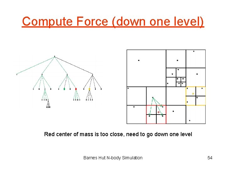
Compute Force (down one level) Red center of mass is too close, need to go down one level Barnes Hut N-body Simulation 54

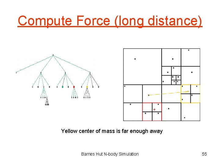
Compute Force (long distance) Yellow center of mass is far enough away Barnes Hut N-body Simulation 55

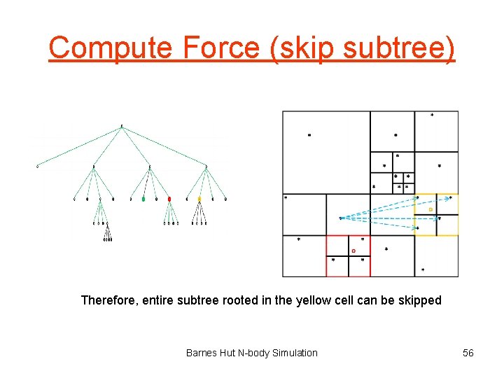
Compute Force (skip subtree) Therefore, entire subtree rooted in the yellow cell can be skipped Barnes Hut N-body Simulation 56

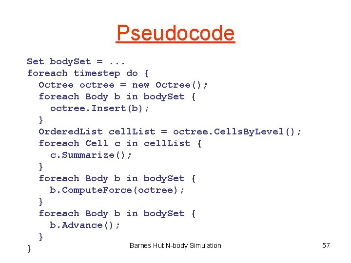
Pseudocode Set body. Set =. . . foreach timestep do { Octree octree = new Octree(); foreach Body b in body. Set { octree. Insert(b); } Ordered. List cell. List = octree. Cells. By. Level(); foreach Cell c in cell. List { c. Summarize(); } foreach Body b in body. Set { b. Compute. Force(octree); } foreach Body b in body. Set { b. Advance(); } Barnes Hut N-body Simulation } 57

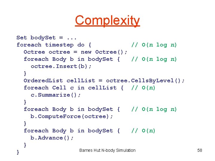
Complexity Set body. Set =. . . foreach timestep do { // O(n log n) Octree octree = new Octree(); foreach Body b in body. Set { // O(n log n) octree. Insert(b); } Ordered. List cell. List = octree. Cells. By. Level(); foreach Cell c in cell. List { // O(n) c. Summarize(); } foreach Body b in body. Set { // O(n log n) b. Compute. Force(octree); } foreach Body b in body. Set { // O(n) b. Advance(); } Barnes Hut N-body Simulation } 58

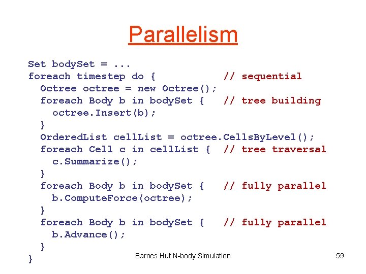
Parallelism Set body. Set =. . . foreach timestep do { // sequential Octree octree = new Octree(); foreach Body b in body. Set { // tree building octree. Insert(b); } Ordered. List cell. List = octree. Cells. By. Level(); foreach Cell c in cell. List { // tree traversal c. Summarize(); } foreach Body b in body. Set { // fully parallel b. Compute. Force(octree); } foreach Body b in body. Set { // fully parallel b. Advance(); } Barnes Hut N-body Simulation } 59

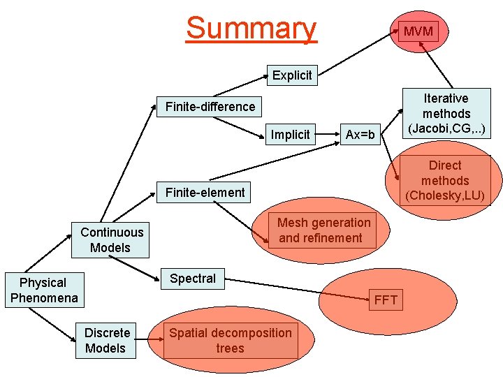
Summary MVM Explicit Finite-difference Implicit Ax=b Direct methods (Cholesky, LU) Finite-element Mesh generation and refinement Continuous Models Spectral Physical Phenomena FFT Discrete Models Iterative methods (Jacobi, CG, . . ) Spatial decomposition trees

Summary (contd. ) • Some key computational science algorithms and data structures – MVM: • explicit finite-difference methods for ode’s, iterative linear solvers, finiteelement methods • both dense and sparse matrices – stencil computations: • finite-difference methods for pde’s • dense matrices – A=LU: • direct methods for solving linear systems: factorization • usually only dense matrices • high-performance factorization codes use MMM as a kernel – mesh generation and refinement • finite-element methods • Graphs – tree building and traversals • n-body methods • Trees

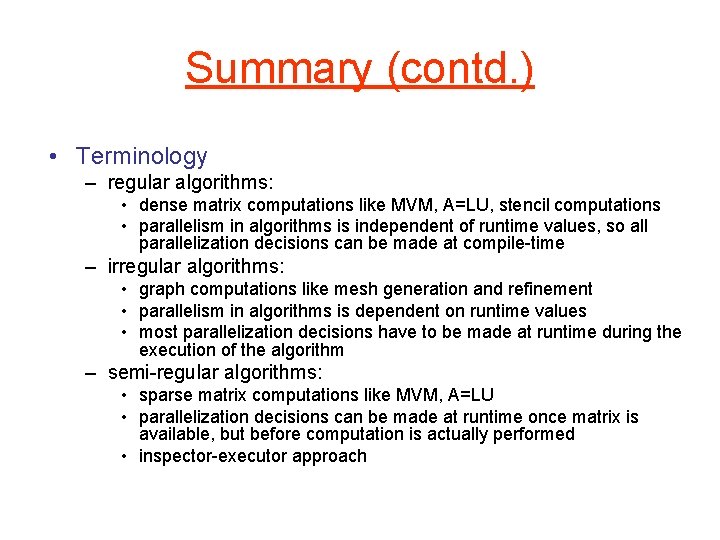
Summary (contd. ) • Terminology – regular algorithms: • dense matrix computations like MVM, A=LU, stencil computations • parallelism in algorithms is independent of runtime values, so all parallelization decisions can be made at compile-time – irregular algorithms: • graph computations like mesh generation and refinement • parallelism in algorithms is dependent on runtime values • most parallelization decisions have to be made at runtime during the execution of the algorithm – semi-regular algorithms: • sparse matrix computations like MVM, A=LU • parallelization decisions can be made at runtime once matrix is available, but before computation is actually performed • inspector-executor approach