Solving recurrence equations 5 techniques for solving recurrence

Solving recurrence equations • 5 techniques for solving recurrence equations: – Recursion tree – Iteration method – Induction (Guess and Test) – Master Theorem (master method) – Characteristic equations • We concentrate on the recursion tree method (others in the book) 10/16/2021 cutler: divide & conquer 1

Deriving the count using the recursion tree method • Recursion trees provide a convenient way to represent the unrolling of recursive algorithm • It is not a formal proof but a good technique to compute the count. • Once the tree is generated, each node contains its “non recursive number of operations” t(n) or Direct. Solution. Count • The count is derived by summing the “non recursive number of operations” of all the nodes in the tree • For convenience we usually compute the sum for all nodes at each given depth, and then sum these sums over all depths. 10/16/2021 cutler: divide & conquer 2

Building the recursion tree • The initial recursion tree has a single node containing two fields: – The recursive call, (for example Factorial(n)) and – the corresponding count T(n). • The tree is generated by: – unrolling the recursion of the node depth 0, – then unrolling the recursion for the nodes at depth 1, etc. • The recursion is unrolled as long as the size of the recursive call is greater than Direct. Solution. Size 10/16/2021 cutler: divide & conquer 3

Building the recursion tree • When the “recursion is unrolled”, each current leaf node is substituted by a subtree containing a root and a child for each recursive call done by the algorithm. – The root of the subtree contains the recursive call, and the corresponding “non recursive count”. – Each child node contains a recursive call, and its corresponding count. • The unrolling continues, until the “size” in the recursive call is Direct. Solution. Size • Nodes with a call of Direct. Solution. Size, are not “unrolled”, and their count is replaced by Direct. Solution. Count 10/16/2021 cutler: divide & conquer 4

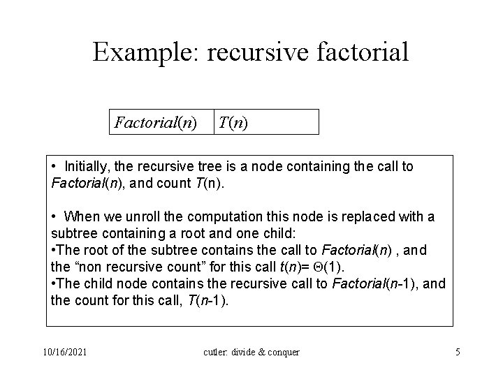
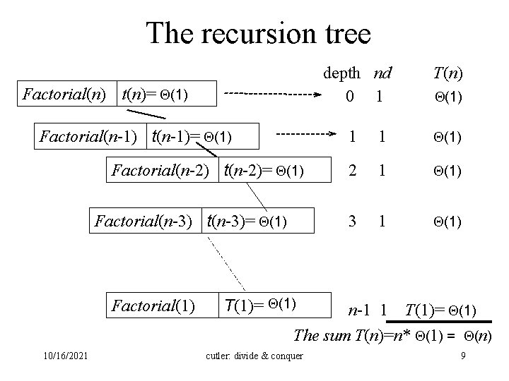
Example: recursive factorial Factorial(n) T(n) • Initially, the recursive tree is a node containing the call to Factorial(n), and count T(n). • When we unroll the computation this node is replaced with a subtree containing a root and one child: • The root of the subtree contains the call to Factorial(n) , and the “non recursive count” for this call t(n)= (1). • The child node contains the recursive call to Factorial(n-1), and the count for this call, T(n-1). 10/16/2021 cutler: divide & conquer 5

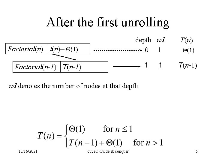
After the first unrolling depth nd 0 1 Factorial(n) t(n)= (1) 1 Factorial(n-1) T(n-1) 1 T(n) (1) T(n-1) nd denotes the number of nodes at that depth 10/16/2021 cutler: divide & conquer 6

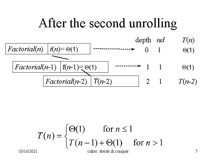
After the second unrolling Factorial(n) t(n)= (1) Factorial(n-1) t(n-1)= (1) Factorial(n-2) T(n-2) 10/16/2021 cutler: divide & conquer depth nd 0 1 T(n) 1 1 (1) 2 1 T(n-2) (1) 7

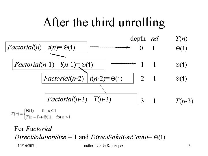
After the third unrolling Factorial(n) t(n)= (1) Factorial(n-1) t(n-1)= (1) Factorial(n-2) t(n-2)= (1) Factorial(n-3) T(n-3) depth nd 0 1 T(n) 1 1 (1) 2 1 (1) 3 1 T(n-3) (1) For Factorial Direct. Solution. Size = 1 and Direct. Solution. Count= (1) 10/16/2021 cutler: divide & conquer 8

The recursion tree Factorial(n) t(n)= (1) Factorial(n-1) t(n-1)= (1) Factorial(n-2) t(n-2)= (1) Factorial(n-3) t(n-3)= (1) Factorial(1) 10/16/2021 depth nd 0 1 T(n) 1 1 (1) 2 1 (1) 3 1 (1) T(1)= (1) n-1 1 T(1)= (1) The sum T(n)=n* (1) = (n) cutler: divide & conquer 9

Divide and Conquer • Basic idea: divide a problem into smaller portions, solve the smaller portions and combine the results. • Name some algorithms you already know that employ this technique. • D&C is a top down approach. Often, you use recursion to implement D&C algorithms. • The following is an “outline” of a divide and conquer algorithm 10/16/2021 cutler: divide & conquer 10

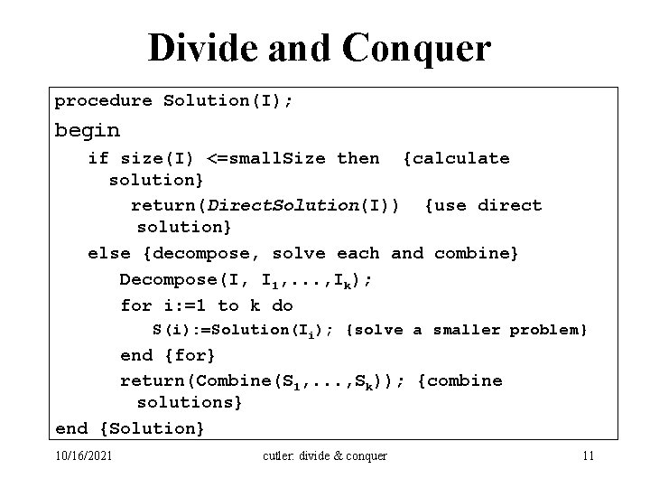
Divide and Conquer procedure Solution(I); begin if size(I) <=small. Size then {calculate solution} return(Direct. Solution(I)) {use direct solution} else {decompose, solve each and combine} Decompose(I, I 1, . . . , Ik); for i: =1 to k do S(i): =Solution(Ii); {solve a smaller problem} end {for} return(Combine(S 1, . . . , Sk)); {combine solutions} end {Solution} 10/16/2021 cutler: divide & conquer 11

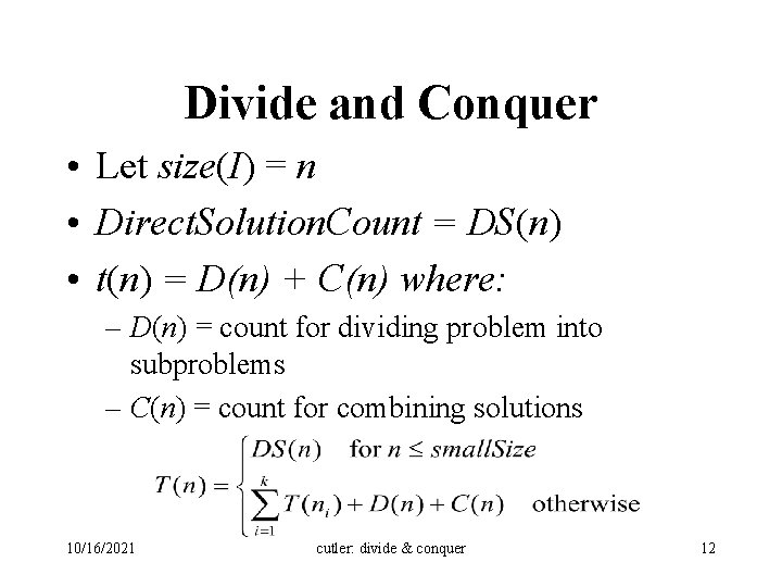
Divide and Conquer • Let size(I) = n • Direct. Solution. Count = DS(n) • t(n) = D(n) + C(n) where: – D(n) = count for dividing problem into subproblems – C(n) = count for combining solutions 10/16/2021 cutler: divide & conquer 12

Divide and Conquer • Main advantages – Simple code – Often efficient algorithms – Suitable for parallel computation 10/16/2021 cutler: divide & conquer 13

Binary search • Assumption - the list S[low…high] is sorted, and x is the search key • If the search key x is in the list, x==S[i], and the index i is returned. • If x is not in the list a No. Such. Key is returned • Book’s version: returns an index i where x would be inserted into the sorted list 10/16/2021 cutler: divide & conquer 14

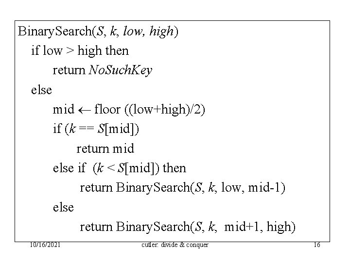
Binary search • The problem is divided into 3 subproblems: x=S[mid], xÎ S[low, . . , mid 1], xÎ S[mid+1, . . , high] • The first case x=S[mid]) is easily solved • The other cases xÎ S[low, . . , mid-1], or xÎ S[mid+1, . . , high] require a recursive call 10/16/2021 cutler: divide & conquer 15

Binary. Search(S, k, low, high) if low > high then return No. Such. Key else mid floor ((low+high)/2) if (k == S[mid]) return mid else if (k < S[mid]) then return Binary. Search(S, k, low, mid-1) else return Binary. Search(S, k, mid+1, high) 10/16/2021 cutler: divide & conquer 16

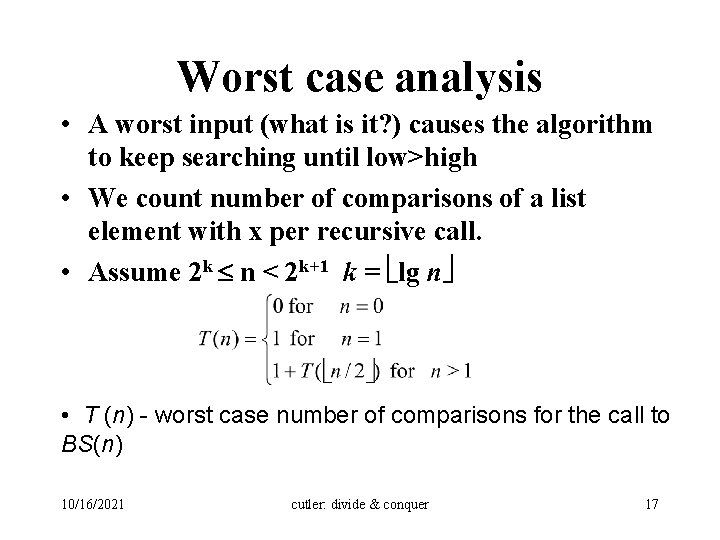
Worst case analysis • A worst input (what is it? ) causes the algorithm to keep searching until low>high • We count number of comparisons of a list element with x per recursive call. • Assume 2 k n < 2 k+1 k = ëlg nû • T (n) - worst case number of comparisons for the call to BS(n) 10/16/2021 cutler: divide & conquer 17

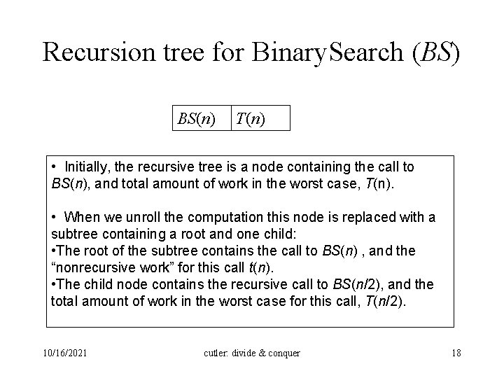
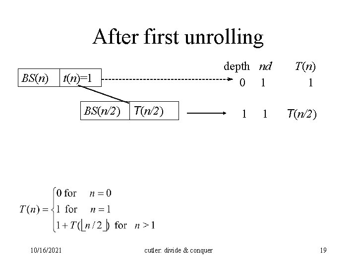
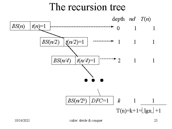
Recursion tree for Binary. Search (BS) BS(n) T(n) • Initially, the recursive tree is a node containing the call to BS(n), and total amount of work in the worst case, T(n). • When we unroll the computation this node is replaced with a subtree containing a root and one child: • The root of the subtree contains the call to BS(n) , and the “nonrecursive work” for this call t(n). • The child node contains the recursive call to BS(n/2), and the total amount of work in the worst case for this call, T(n/2). 10/16/2021 cutler: divide & conquer 18

After first unrolling BS(n) t(n)=1 BS(n/2) 10/16/2021 depth nd 0 1 T(n/2) cutler: divide & conquer 1 1 T(n) 1 T(n/2) 19

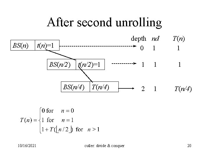
After second unrolling BS(n) t(n)=1 BS(n/2) t(n/2)=1 BS(n/4) 10/16/2021 T(n/4) cutler: divide & conquer depth nd 0 1 T(n) 1 1 2 1 T(n/4) 20

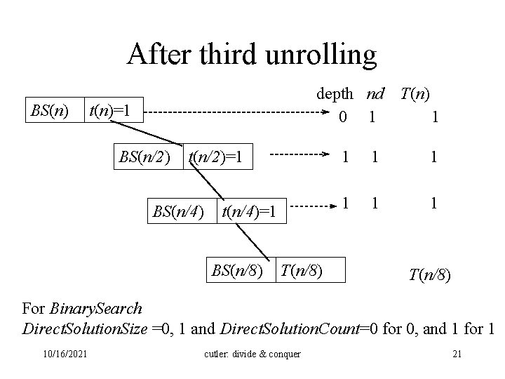
After third unrolling BS(n) depth nd 0 1 t(n)=1 BS(n/2) t(n/2)=1 BS(n/4) t(n/4)=1 BS(n/8) T(n) 1 1 1 1 T(n/8) For Binary. Search Direct. Solution. Size =0, 1 and Direct. Solution. Count=0 for 0, and 1 for 1 10/16/2021 cutler: divide & conquer 21

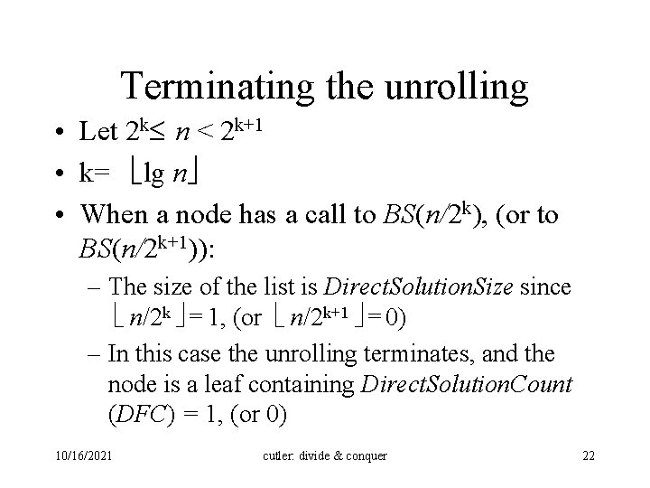
Terminating the unrolling • Let 2 k n < 2 k+1 • k= lg n • When a node has a call to BS(n/2 k), (or to BS(n/2 k+1)): – The size of the list is Direct. Solution. Size since n/2 k = 1, (or n/2 k+1 = 0) – In this case the unrolling terminates, and the node is a leaf containing Direct. Solution. Count (DFC) = 1, (or 0) 10/16/2021 cutler: divide & conquer 22

The recursion tree depth nd BS(n) t(n)=1 BS(n/2) t(n/2)=1 BS(n/4) t(n/4)=1 BS(n/2 k) DFC=1 T(n) 0 1 1 1 2 1 1 k 1 1 T(n)=k+1= lgn +1 10/16/2021 cutler: divide & conquer 23

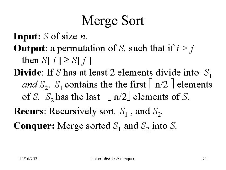
Merge Sort Input: S of size n. Output: a permutation of S, such that if i > j then S[ i ] S[ j ] Divide: If S has at least 2 elements divide into S 1 and S 2. S 1 contains the first n/2 elements of S. S 2 has the last n/2 elements of S. Recurs: Recursively sort S 1 , and S 2. Conquer: Merge sorted S 1 and S 2 into S. 10/16/2021 cutler: divide & conquer 24

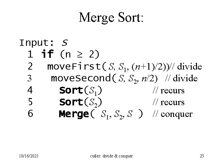
Merge Sort: Input: S 1 if (n 2) 2 move. First( S, S 1, (n+1)/2))// divide 3 move. Second( S, S 2, n/2) // divide 4 Sort(S 1) // recurs 5 Sort(S 2) // recurs 6 Merge( S 1, S 2, S ) // conquer 10/16/2021 cutler: divide & conquer 25

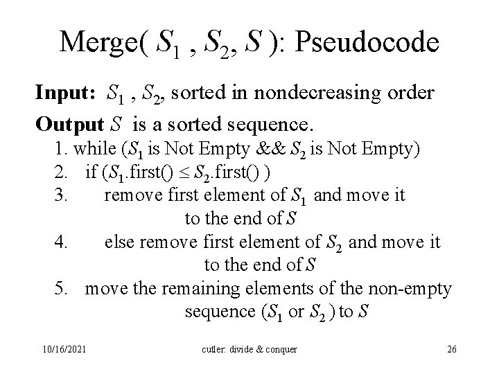
Merge( S 1 , S 2, S ): Pseudocode Input: S 1 , S 2, sorted in nondecreasing order Output S is a sorted sequence. 1. while (S 1 is Not Empty && S 2 is Not Empty) 2. if (S 1. first() S 2. first() ) 3. remove first element of S 1 and move it to the end of S 4. else remove first element of S 2 and move it to the end of S 5. move the remaining elements of the non-empty sequence (S 1 or S 2 ) to S 10/16/2021 cutler: divide & conquer 26

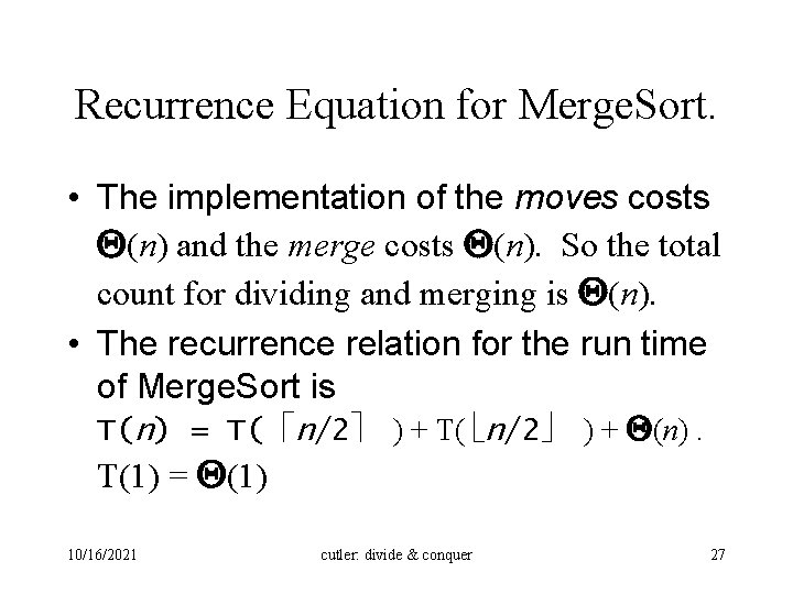
Recurrence Equation for Merge. Sort. • The implementation of the moves costs Q(n) and the merge costs Q(n). So the total count for dividing and merging is Q(n). • The recurrence relation for the run time of Merge. Sort is T(n) = T( n/2 ) + Q(n). T(1) = Q(1) 10/16/2021 cutler: divide & conquer 27

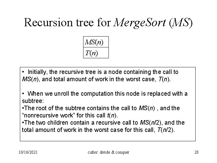
Recursion tree for Merge. Sort (MS) MS(n) T(n) • Initially, the recursive tree is a node containing the call to MS(n), and total amount of work in the worst case, T(n). • When we unroll the computation this node is replaced with a subtree: • The root of the subtree contains the call to MS(n) , and the “nonrecursive work” for this call t(n). • The two children contain a recursive call to MS(n/2), and the total amount of work in the worst case for this call, T(n/2). 10/16/2021 cutler: divide & conquer 28

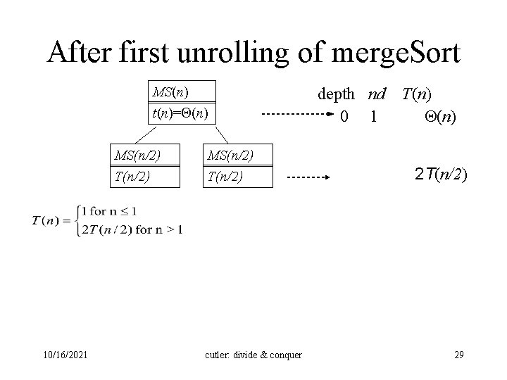
After first unrolling of merge. Sort MS(n) t(n)= (n) MS(n/2) T(n/2) 10/16/2021 MS(n/2) T(n/2) cutler: divide & conquer depth nd 0 1 T(n) 2 T(n/2) 29

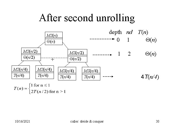
After second unrolling depth nd 0 1 MS(n) MS(n/2) MS(n/4) T(n/4) 10/16/2021 + MS(n/4) T(n/4) MS(n/2) MS(n/4) T(n/4) cutler: divide & conquer 1 2 T(n) (n) 4 T(n/4) 30

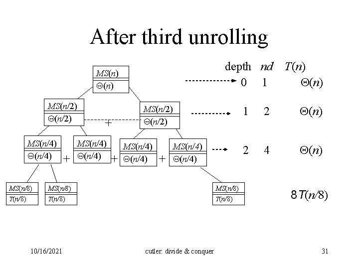
After third unrolling depth nd 0 1 MS(n) MS(n/2) MS(n/4) MS(n/8) T(n/8) + + MS(n/4) + MS(n/2) MS(n/4) + MS(n/4) MS(n/8) T(n/8) 10/16/2021 MS(n/8) T(n/8) cutler: divide & conquer T(n) 1 2 (n) 2 4 (n) 8 T(n/8) 31

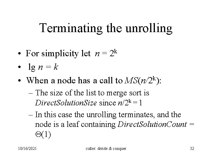
Terminating the unrolling • For simplicity let n = 2 k • lg n = k • When a node has a call to MS(n/2 k): – The size of the list to merge sort is Direct. Solution. Size since n/2 k = 1 – In this case the unrolling terminates, and the node is a leaf containing Direct. Solution. Count = (1) 10/16/2021 cutler: divide & conquer 32

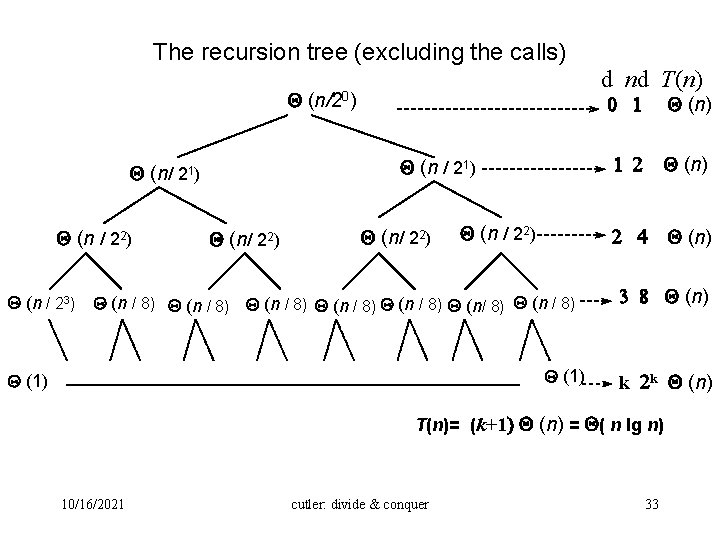
The recursion tree (excluding the calls) d nd T(n) Q (n/20) Q (n / 21) Q (n / 22) Q (n / 23) Q (n/ 22) Q (n / 8) Q (n / 8) Q (n / 8) Q (1) 0 1 Q (n) 1 2 Q (n) 2 4 Q (n) 3 8 Q (n) k 2 k Q (n) T(n)= (k+1) Q (n) = Q( n lg n) 10/16/2021 cutler: divide & conquer 33

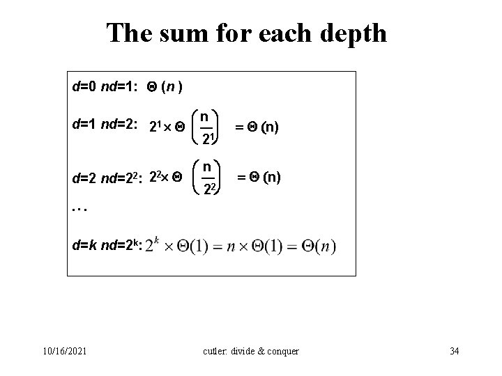
The sum for each depth d=0 nd=1: Q (n ) n d=1 nd=2: 21 ´ Q æç ö÷ è 21ø = Q (n) æ nö Q ç ÷ è 22ø = Q (n) d=2 nd=22: 22´ . . . d=k nd=2 k: 10/16/2021 cutler: divide & conquer 34