Solving problems by searching Chapter 3 Continue 1
Solving problems by searching Chapter 3 /Continue 1
Tree search algorithms n Basic idea: n n Exploration of state space by generating successors of already-explored states (a. k. a. expanding states). Every states is evaluated: is it a goal state? 2
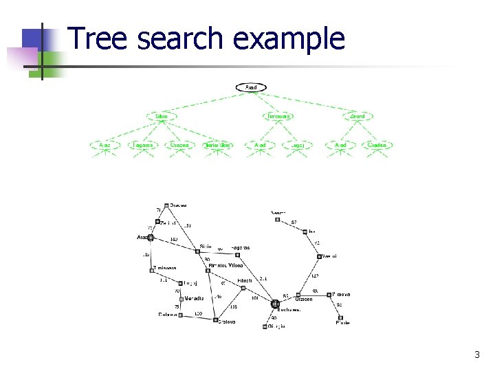
Tree search example 3
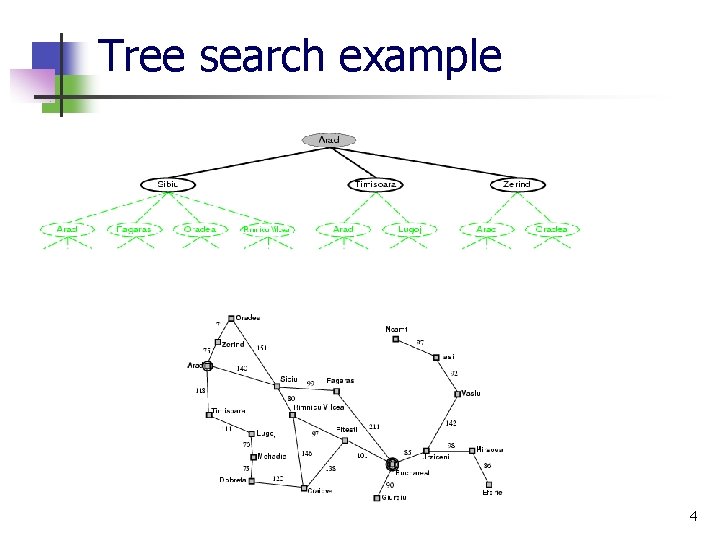
Tree search example 4

Tree search example 5
Infrastructure for search algorithms n Search algorithms require a data structure to keep track of the search tree that is being constructed. For each node n of the tree, we have a structure that contains four components: 1 - n. STATE: the state in the state space to which the node corresponds; 2 - n. PARENT: the node in the search tree that generated this node; 3 - n. ACTION: the action that was applied to the parent to generate the node; 4 - n. PATH-COST: the cost, traditionally denoted by g(n), of the path from the initial state to the node, as indicated by the parent pointers. 6
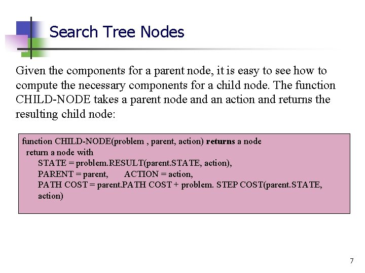
Search Tree Nodes Given the components for a parent node, it is easy to see how to compute the necessary components for a child node. The function CHILD-NODE takes a parent node and an action and returns the resulting child node: function CHILD-NODE(problem , parent, action) returns a node return a node with STATE = problem. RESULT(parent. STATE, action), PARENT = parent, ACTION = action, PATH COST = parent. PATH COST + problem. STEP COST(parent. STATE, action) 7
Search Tree Nodes n n Notice how the PARENT pointers string the nodes together into a tree structure. The SOLUTION function is used to return the sequence of actions obtained by following parent pointers back to the root (in case a goal node is found). 8
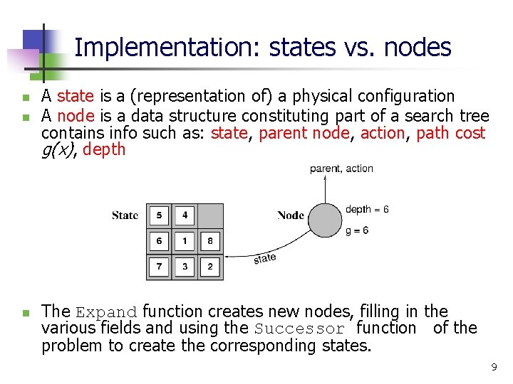
Implementation: states vs. nodes n n n A state is a (representation of) a physical configuration A node is a data structure constituting part of a search tree contains info such as: state, parent node, action, path cost g(x), depth The Expand function creates new nodes, filling in the various fields and using the Successor function of the problem to create the corresponding states. 9
states vs. nodes n n Thus, nodes are on particular paths, as defined by PARENT pointers, whereas states are not. Furthermore, two different nodes can contain the same world state if that state is generated via two different search paths. 10
Frontiers and QUEUE Data Structure n n Nodes need somewhere to be put into. The frontier needs to be stored in such a way that the search algorithm can easily choose the next node to expand according to its preferred strategy. QUEUE is the appropriate data structure for this is with the following operations : o EMPTY? ( queue) returns true only if there are no more elements in the queue. o POP(queue) removes the first element of the queue and returns it. o INSERT(element, queue) inserts an element and returns the resulting queue. 11
A QUEUE Data Structure Queues are characterized by the order in which they store the inserted nodes. Three common variants exists: n FIFO queue, which pops the oldest element of the queue; n LIFO queue (a. k. a a stack), which pops the newest element n PRIORITY queue, which pops the element of the queue with the highest priority according to some ordering function. 12
Explored set and Hash Tables n n The explored set can be implemented with a hash table to allow efficient checking for repeated states. With a good implementation, insertion and lookup can be done in roughly constant time no matter how many states are stored. 13
Search strategies: Measuring problem-solving performance n n A search strategy is defined by picking the order of node expansion Strategies are evaluated along the following dimensions: n n n completeness: does it always find a solution if one exists? time complexity: number of nodes generated space complexity: maximum number of nodes in memory optimality: does it always find a least-cost solution? Time and space complexity are always considered with respect to some measure of the problem difficulty. In theoretical computer science, the typical measure: is the size of the state space graph. 14
Measuring problem-solving performance n n n This is appropriate when the graph is an explicit data structure that is input to the search program (e. g. the map of Romania ). In AI, the graph is often represented implicitly by the initial state, actions, and transition model. For these reasons, complexity is expressed in terms of three quantities: n n n b: branching factor of the search tree ( i. e. , maximum number of successors of any node ) d: the depth of the shallowest goal node (i. e. , the number of steps along the path from the root) m: maximum depth of the state space ( i. e. , the maximum length of any path in the state space (may be ∞) 15
n n Time is often measured in terms of the number of nodes generated during the search. Space is measured in terms of the maximum number of nodes stored in memory. n 16
Effectiveness of a Search Algorithm n n n To assess the effectiveness of a search algorithm, we can consider just the search cost— which typically depends on the time complexity but can also include a term for memory usage We can use the total cost, which combines the search cost and the path cost of the solution found. Example: For the problem of finding a route from Arad to Bucharest, the search cost is the amount of time taken by the search and the solution cost is the total length of the path 17
UNINFORMED SEARCH STRATEGIES n n Un-informed Search (also called blind search). The term means that the strategies have no additional information about states other than that provided in the problem definition. All that these stategies can do is to generate successors and distinguish a goal state from a non-goal state. All search strategies are distinguished by the order in which nodes are expanded. On the contrary, strategies that know whether a non-goal state is “non promising" than another are called informed search or heuristic search strategies. 18
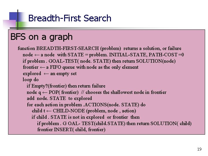
Breadth-First Search BFS on a graph function BREADTH-FIRST-SEARCH (problem) returns a solution, or failure node ← a node with STATE = problem. INITIAL-STATE, PATH-COST =0 if problem. GOAL-TEST( node. STATE) then return SOLUTION(node) frontier ← a FIFO queue with node as the only element explored ← an empty set loop do if Empty? (frontier) then return failure node q ← POP( frontier) // chooses the shallowest node in frontier add node. STATE to explored for each action in problem. ACTIONS(node. STATE) do child t ← CHILD-NODE (problem, node , action) if child. STATE is not in explored or frontier then if problem. G OAL- TEST(child. STATE) then return SOLUTION( child) frontier INSERT( child, frontier) 19
Evaluating BFS Algorithm n Left for “Self Study” 20
About BFS n n Two lessons can be learned from BFS algorithm: 1 - The memory requirements are a bigger problem for breadth first search than is the execution time. 2 - The time is still a major factor. If a problem has a solution at depth 16, then (given our assumptions) it will take about 350 years for breadth-first search for indeed any uninformed search) to find it. In general, exponential-complexity search problems cannot be solved by uninformed methods for any but the smallest instances. 21
Uniform-cost search n n A simple extension to BFS is the one that expands the node n with the lowest path cost g(n). This is done by storing the frontier as a priority queue ordered by g. The algorithm is shown next. In addition to the ordering of the queue by path cost, there are two other significant differences from BFS : 1. The goal test is applied to a node when it is selected for expansion (as in the generic graph-search algorithm) rather than when it is first generated. 2. A test is added in case a better path is found to a node currently on the frontier. 22
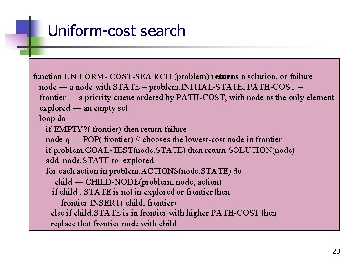
Uniform-cost search function UNIFORM- COST-SEA RCH (problem) returns a solution, or failure node ← a node with STATE = problem. INITIAL-STATE, PATH-COST = frontier ← a priority queue ordered by PATH-COST, with node as the only element explored ← an empty set loop do if EMPTY? ( frontier) then return failure node q ← POP( frontier) // chooses the lowest-cost node in frontier if problem. GOAL-TEST(node. STATE) then return SOLUTION(node) add node. STATE to explored for each action in problem. ACTIONS(node. STATE) do child ← CHILD-NODE(problern, node, action) if child. STATE is not in explored or frontier then frontier INSERT( child, frontier) else if child. STATE is in frontier with higher PATH-COST then replace that frontier node with child 23
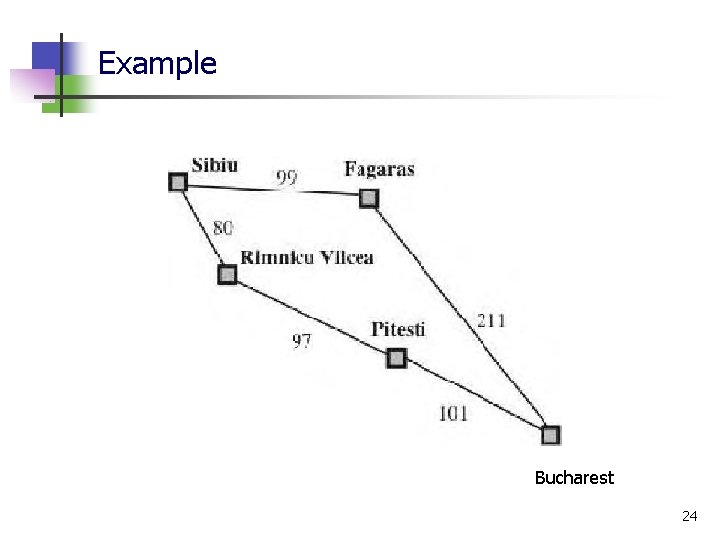
Example Bucharest 24
General Observations n n n Uniform-cost search is guided by path costs rather than depths, so its complexity is not easily characterized in terms of b and d. When all step costs are the same, uniform-cost search is similar to breadth-first search, except that the latter stops as soon as it generates a goal, whereas uniform-cost search examines all the nodes at the goal's depth to see if one has a lower cost. Thus uniform-cost search does strictly more work by expanding nodes at depth d unnecessarily. 25
Depth-First Search n n n DFS always expands the deepest node in the current frontier of the search tree. The search proceeds immediately to the deepest level of the search tree, where the nodes have no successors. As those nodes are expanded, they are dropped from the frontier, so then the search "backs up" to the next deepest node that still has unexplored successors. The depth-first search algorithm is an instance of the graph-search algorithm. Whereas breadth-first-search uses a FIFO queue, depth-first search uses a Stack. This means that the most recently generated node is chosen for expansion. This must be the deepest unexpanded node because it is one deeper than its parent—which, in turn, was the deepest unexpanded node when it was selected. 26
Self Study n n Difference between depth-first graph search and depth-first tree search. Difference between depth-first search and breadth-first search. 27
Recursive Depth Limited Search n As an alternative to the GRAPH-SEARCH-style implementation, it is common to implement depth-first search with a recursive function that calls itself on each of its children in turn. A recursive depth-first algorithm incorporating a depth limit is shown next. 28
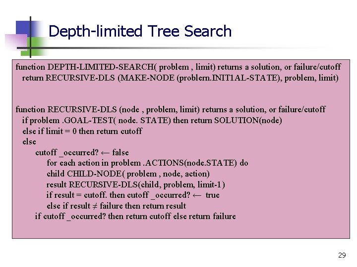
Depth-limited Tree Search function DEPTH-LIMITED-SEARCH( problem , limit) returns a solution, or failure/cutoff return RECURSIVE-DLS (MAKE-NODE (problern. INIT 1 AL-STATE), problem, limit) function RECURSIVE-DLS (node , problem, limit) returns a solution, or failure/cutoff if problem. GOAL-TEST( node. STATE) then return SOLUTION(node) else if limit = 0 then return cutoff else cutoff _occurred? ← false for each action in problem. ACTIONS(node. STATE) do child CHILD-NODE( problem , node, action) result RECURSIVE-DLS(child, problem, limit-1) if result = cutoff. then cutoff _occurred? ← true else if result ≠ failure then return result if cutoff _occurred? then return cutoff else return failure 29
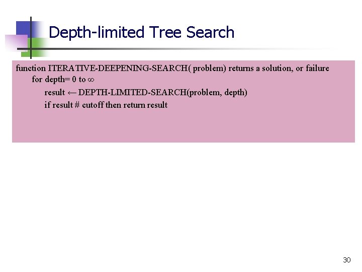
Depth-limited Tree Search function ITERATIVE-DEEPENING-SEARCH( problem) returns a solution, or failure for depth= 0 to ∞ result ← DEPTH-LIMITED-SEARCH(problem, depth) if result # cutoff then return result 30
Self Study n Comparison between complexity of DFS and DLS. 31
- Slides: 31