Solving Linear Programs The Simplex Method 1 The

Solving Linear Programs: The Simplex Method 1

The Essence • Simplex method is an algebraic procedure • However, its underlying concepts are geometric • Understanding these geometric concepts helps before going into their algebraic equivalents 2

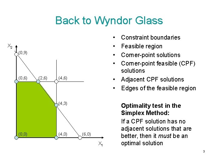
Back to Wyndor Glass • • Constraint boundaries Feasible region Corner-point solutions Corner-point feasible (CPF) solutions • Adjacent CPF solutions • Edges of the feasible region X 2 (0, 9) (0, 6) (2, 6) (4, 3) (0, 0) (4, 0) (6, 0) X 1 Optimality test in the Simplex Method: If a CPF solution has no adjacent solutions that are better, then it must be an optimal solution 3

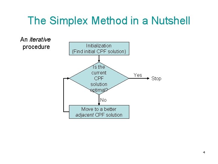
The Simplex Method in a Nutshell An iterative procedure Initialization (Find initial CPF solution) Is the current CPF solution optimal? Yes Stop No Move to a better adjacent CPF solution 4

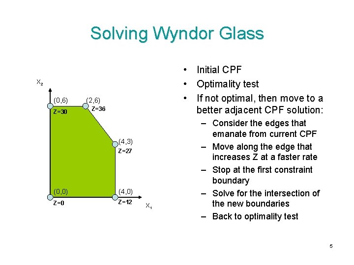
Solving Wyndor Glass • Initial CPF • Optimality test • If not optimal, then move to a better adjacent CPF solution: X 2 (0, 6) Z=30 (2, 6) Z=36 (4, 3) Z=27 (0, 0) (4, 0) Z=0 Z=12 X 1 – Consider the edges that emanate from current CPF – Move along the edge that increases Z at a faster rate – Stop at the first constraint boundary – Solve for the intersection of the new boundaries – Back to optimality test 5

Key Concepts • • • Focus only on CPF solutions An iterative algorithm If possible, use the origin as the initial CPF solution Move always to adjacent CPF solutions Don’t calculate the Z value at adjacent solutions, instead move directly to the one that ‘looks’ better (on the edge with the higher rate of improvement) • Optimality test also looks at the rate of improvement (If all negative, then optimal) 6

‘Language’ of the Simplex Method 7

Initial Assumptions • All constraints are of the form ≤ • All right-hand-side values (bj, j=1, …, m) are positive • We’ll learn how to address other forms later 8

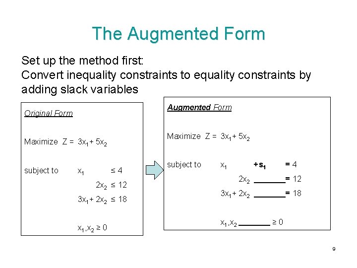
The Augmented Form Set up the method first: Convert inequality constraints to equality constraints by adding slack variables Augmented Form Original Form Maximize Z = 3 x 1+ 5 x 2 subject to x 1 ≤ 4 2 x 2 ≤ 12 3 x 1+ 2 x 2 ≤ 18 x 1, x 2 ≥ 0 subject to x 1 +s 1 =4 2 x 2 = 12 3 x 1+ 2 x 2 = 18 x 1, x 2 ≥ 0 9

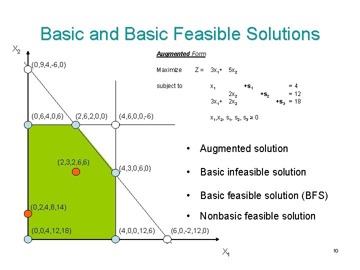
X 2 Basic and Basic Feasible Solutions Augmented Form (0, 9, 4, -6, 0) Maximize Z= subject to 3 x 1+ x 1 +s 1 3 x 1+ (0, 6, 4, 0, 6) (2, 6, 2, 0, 0) 5 x 2 (4, 6, 0, 0, -6) 2 x 2 +s 3 =4 = 12 = 18 x 1, x 2, s 1, s 2, s 3 ≥ 0 • Augmented solution (2, 3, 2, 6, 6) (4, 3, 0, 6, 0) • Basic infeasible solution • Basic feasible solution (BFS) (0, 2, 4, 8, 14) (0, 0, 4, 12, 18) • Nonbasic feasible solution (4, 0, 0, 12, 6) (6, 0, -2, 12, 0) X 1 10

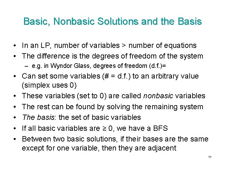
Basic, Nonbasic Solutions and the Basis • In an LP, number of variables > number of equations • The difference is the degrees of freedom of the system – e. g. in Wyndor Glass, degrees of freedom (d. f. )= • Can set some variables (# = d. f. ) to an arbitrary value (simplex uses 0) • These variables (set to 0) are called nonbasic variables • The rest can be found by solving the remaining system • The basis: the set of basic variables • If all basic variables are ≥ 0, we have a BFS • Between two basic solutions, if their bases are the same except for one variable, then they are adjacent 11

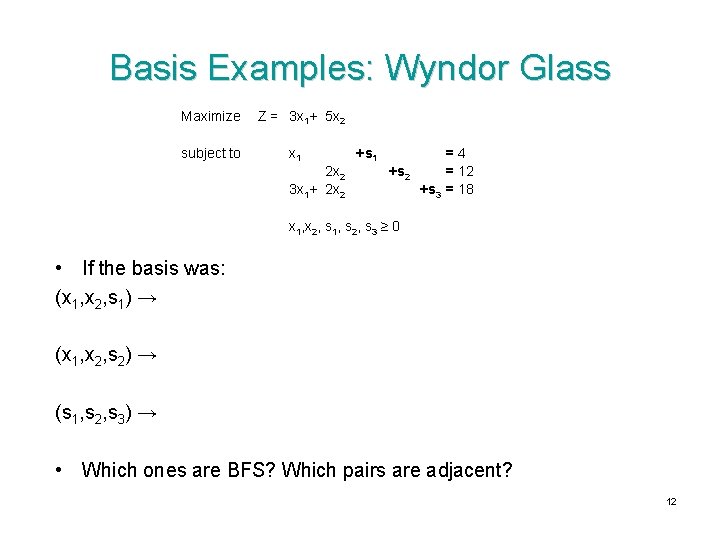
Basis Examples: Wyndor Glass Maximize subject to Z = 3 x 1+ 5 x 2 x 1 2 x 2 3 x 1+ 2 x 2 +s 1 +s 2 =4 = 12 +s 3 = 18 x 1, x 2, s 1, s 2, s 3 ≥ 0 • If the basis was: (x 1, x 2, s 1) → (x 1, x 2, s 2) → (s 1, s 2, s 3) → • Which ones are BFS? Which pairs are adjacent? 12

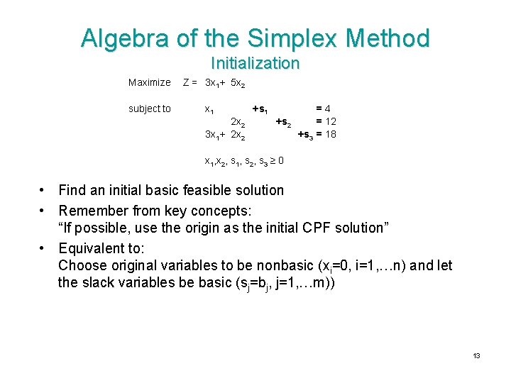
Algebra of the Simplex Method Initialization Maximize subject to Z = 3 x 1+ 5 x 2 x 1 2 x 2 3 x 1+ 2 x 2 +s 1 +s 2 =4 = 12 +s 3 = 18 x 1, x 2, s 1, s 2, s 3 ≥ 0 • Find an initial basic feasible solution • Remember from key concepts: “If possible, use the origin as the initial CPF solution” • Equivalent to: Choose original variables to be nonbasic (xi=0, i=1, …n) and let the slack variables be basic (sj=bj, j=1, …m)) 13

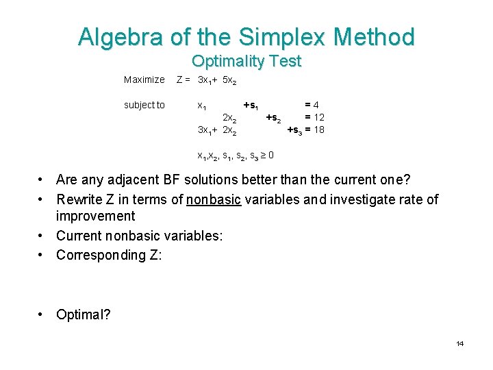
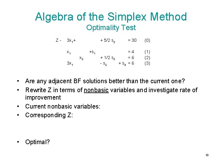
Algebra of the Simplex Method Optimality Test Maximize subject to Z = 3 x 1+ 5 x 2 x 1 2 x 2 3 x 1+ 2 x 2 +s 1 +s 2 =4 = 12 +s 3 = 18 x 1, x 2, s 1, s 2, s 3 ≥ 0 • Are any adjacent BF solutions better than the current one? • Rewrite Z in terms of nonbasic variables and investigate rate of improvement • Current nonbasic variables: • Corresponding Z: • Optimal? 14

Algebra of the Simplex Method Step 1 of Iteration 1: Direction of Movement Maximize subject to Z = 3 x 1+ 5 x 2 x 1 +s 1 2 x 2 3 x 1+ 2 x 2 +s 2 =4 = 12 +s 3 = 18 x 1, x 2, s 1, s 2, s 3 ≥ 0 • Which edge to move on? • Determine the direction of movement by selecting the entering variable (variable ‘entering’ the basis) • Choose the direction of steepest ascent – x 1: Rate of improvement in Z = – x 2: Rate of improvement in Z = • Entering basic variable = 15

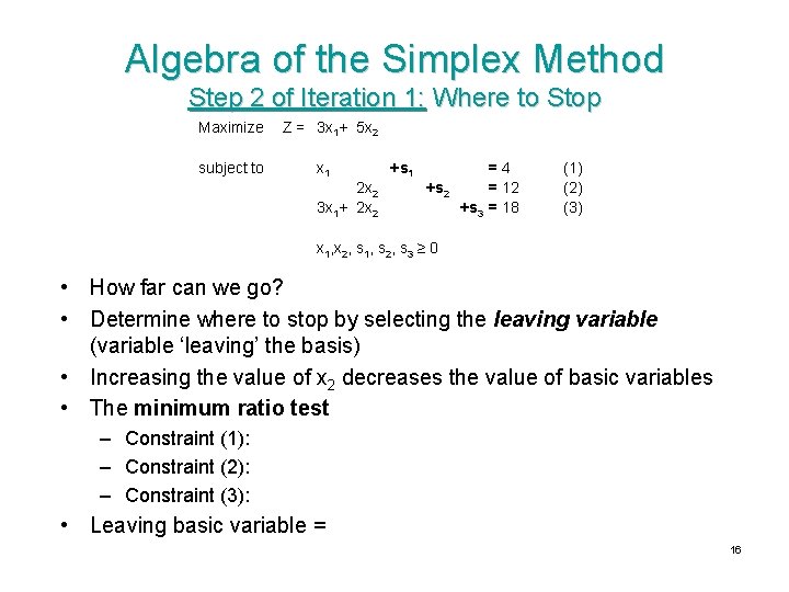
Algebra of the Simplex Method Step 2 of Iteration 1: Where to Stop Maximize subject to Z = 3 x 1+ 5 x 2 x 1 2 x 2 3 x 1+ 2 x 2 +s 1 +s 2 =4 = 12 +s 3 = 18 (1) (2) (3) x 1, x 2, s 1, s 2, s 3 ≥ 0 • How far can we go? • Determine where to stop by selecting the leaving variable (variable ‘leaving’ the basis) • Increasing the value of x 2 decreases the value of basic variables • The minimum ratio test – Constraint (1): – Constraint (2): – Constraint (3): • Leaving basic variable = 16

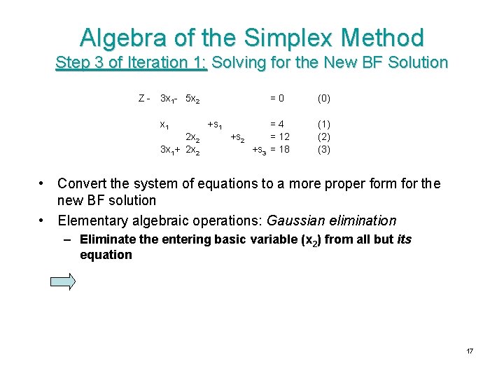
Algebra of the Simplex Method Step 3 of Iteration 1: Solving for the New BF Solution Z- 3 x 1 - 5 x 2 x 1 2 x 2 3 x 1+ 2 x 2 =0 +s 1 +s 2 =4 = 12 +s 3 = 18 (0) (1) (2) (3) • Convert the system of equations to a more proper form for the new BF solution • Elementary algebraic operations: Gaussian elimination – Eliminate the entering basic variable (x 2) from all but its equation 17

Algebra of the Simplex Method Optimality Test Z- 3 x 1+ + 5/2 s 2 x 1 +s 1 x 2 3 x 1 + 1/2 s 2 - s 2 = 30 =4 =6 + s 3 = 6 (0) (1) (2) (3) • Are any adjacent BF solutions better than the current one? • Rewrite Z in terms of nonbasic variables and investigate rate of improvement • Current nonbasic variables: • Corresponding Z: • Optimal? 18

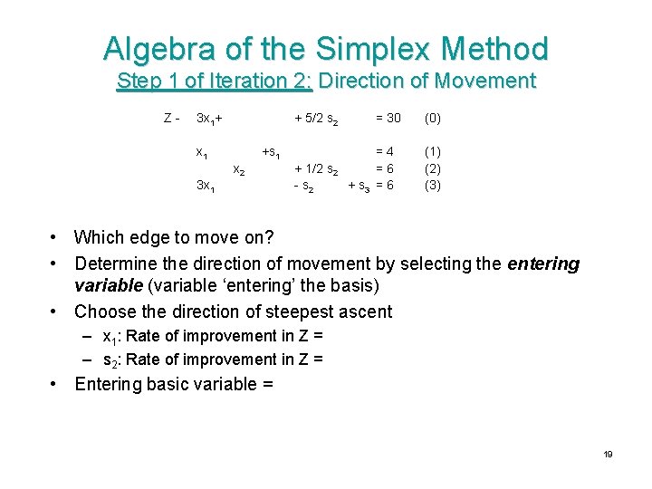
Algebra of the Simplex Method Step 1 of Iteration 2: Direction of Movement Z- 3 x 1+ + 5/2 s 2 x 1 +s 1 x 2 3 x 1 + 1/2 s 2 - s 2 = 30 =4 =6 + s 3 = 6 (0) (1) (2) (3) • Which edge to move on? • Determine the direction of movement by selecting the entering variable (variable ‘entering’ the basis) • Choose the direction of steepest ascent – x 1: Rate of improvement in Z = – s 2: Rate of improvement in Z = • Entering basic variable = 19

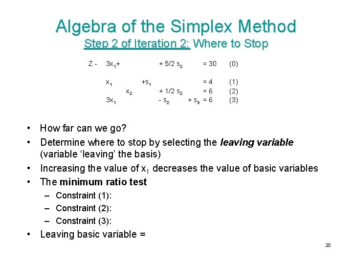
Algebra of the Simplex Method Step 2 of Iteration 2: Where to Stop Z- 3 x 1+ + 5/2 s 2 x 1 +s 1 x 2 3 x 1 + 1/2 s 2 - s 2 = 30 =4 =6 + s 3 = 6 (0) (1) (2) (3) • How far can we go? • Determine where to stop by selecting the leaving variable (variable ‘leaving’ the basis) • Increasing the value of x 1 decreases the value of basic variables • The minimum ratio test – Constraint (1): – Constraint (2): – Constraint (3): • Leaving basic variable = 20

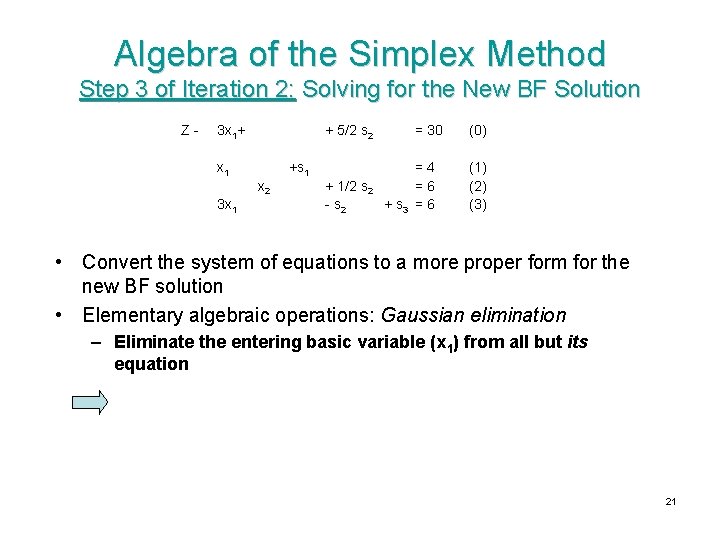
Algebra of the Simplex Method Step 3 of Iteration 2: Solving for the New BF Solution Z- 3 x 1+ + 5/2 s 2 x 1 +s 1 x 2 3 x 1 + 1/2 s 2 - s 2 = 30 =4 =6 + s 3 = 6 (0) (1) (2) (3) • Convert the system of equations to a more proper form for the new BF solution • Elementary algebraic operations: Gaussian elimination – Eliminate the entering basic variable (x 1) from all but its equation 21

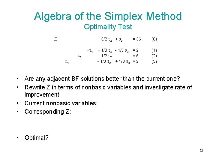
Algebra of the Simplex Method Optimality Test Z + 3/2 s 2 + s 3 +s 1 x 2 x 1 = 36 + 1/3 s 2 - 1/3 s 3 = 2 + 1/2 s 2 =6 - 1/3 s 2 + 1/3 s 3 = 2 (0) (1) (2) (3) • Are any adjacent BF solutions better than the current one? • Rewrite Z in terms of nonbasic variables and investigate rate of improvement • Current nonbasic variables: • Corresponding Z: • Optimal? 22

The Simplex Method in Tabular Form • For convenience in performing the required calculations • Record only the essential information of the (evolving) system of equations in tableaux – Coefficients of the variables – Constants on the right-hand-sides – Basic variables corresponding to equations 23

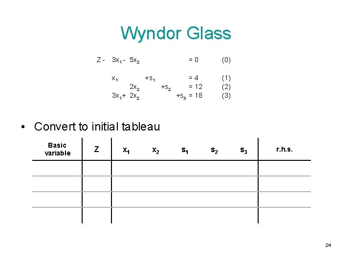
Wyndor Glass Z- 3 x 1 - 5 x 2 x 1 =0 +s 1 2 x 2 3 x 1+ 2 x 2 +s 2 (0) =4 = 12 +s 3 = 18 (1) (2) (3) • Convert to initial tableau Basic variable Z x 1 x 2 s 1 s 2 s 3 r. h. s. 24

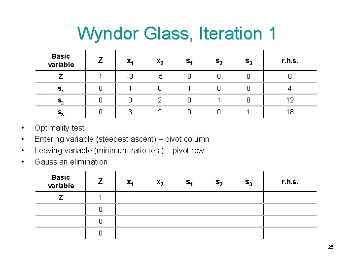
Wyndor Glass, Iteration 1 • • Basic variable Z x 1 x 2 s 1 s 2 s 3 r. h. s. Z 1 -3 -5 0 0 s 1 0 1 0 0 4 s 2 0 0 2 0 12 s 3 0 3 2 0 0 1 18 s 2 s 3 r. h. s. Optimality test Entering variable (steepest ascent) – pivot column Leaving variable (minimum ratio test) – pivot row Gaussian elimination Basic variable Z Z 1 x 2 s 1 0 0 0 25

Wyndor Glass, Iteration 2 • • Basic variable Z x 1 x 2 s 1 s 2 s 3 r. h. s. Z 1 -3 0 0 5/2 0 30 s 1 0 1 0 0 4 x 2 0 0 1/2 0 6 s 3 0 0 -1 1 6 s 2 s 3 r. h. s. Optimality test Entering variable (steepest ascent) – pivot column Leaving variable (minimum ratio test) – pivot row Gaussian elimination Basic variable Z Z 1 x 2 s 1 0 0 0 26

Wyndor Glass, Iteration 3 • • Basic variable Z x 1 x 2 s 1 s 2 s 3 r. h. s. Z 1 0 0 0 3/2 1 36 s 1 0 0 0 1 1/3 -1/3 2 x 2 0 0 1/2 0 6 x 1 0 0 -1/3 2 s 3 r. h. s. Optimality test Entering variable (steepest ascent) – pivot column Leaving variable (minimum ratio test) – pivot row Gaussian elimination Basic variable Z Z 1 x 2 s 1 0 0 0 27

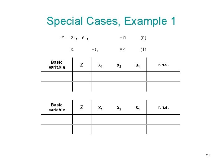
Special Cases, Example 1 Z- 3 x 1 - 5 x 2 x 1 +s 1 =0 (0) =4 (1) Basic variable Z x 1 x 2 s 1 r. h. s. 28

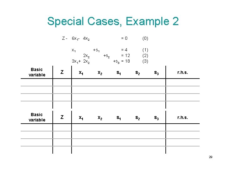
Special Cases, Example 2 Z- 6 x 1 - 4 x 2 x 1 =0 +s 1 2 x 2 3 x 1+ 2 x 2 +s 2 (0) =4 = 12 +s 3 = 18 (1) (2) (3) Basic variable Z x 1 x 2 s 1 s 2 s 3 r. h. s. 29

Special Cases, Example 2, cont’d Basic variable Z x 1 x 2 s 1 s 2 s 3 r. h. s. 30

Special Cases, Example 3 Z- 3 x 1 - 3 x 2 x 1 =0 +s 1 2 x 2 3 x 1+ 2 x 2 Basic variable Z x 1 +s 2 x 2 (0) =4 = 12 +s 3 = 18 s 1 (1) (2) (3) s 2 s 3 r. h. s. 31

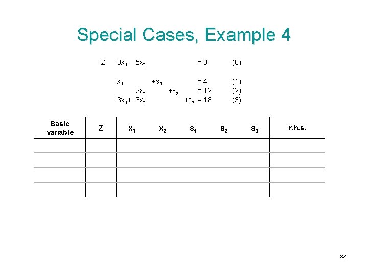
Special Cases, Example 4 Z- 3 x 1 - 5 x 2 x 1 =0 +s 1 2 x 2 3 x 1+ 3 x 2 Basic variable Z x 1 +s 2 x 2 (0) =4 = 12 +s 3 = 18 s 1 (1) (2) (3) s 2 s 3 r. h. s. 32

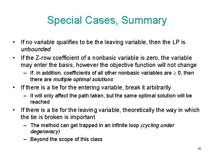
Special Cases, Summary • If no variable qualifies to be the leaving variable, then the LP is unbounded • If the Z-row coefficient of a nonbasic variable is zero, the variable may enter the basis, however the objective function will not change – If, in addition, coefficients of all other nonbasic variables are 0, then there are multiple optimal solutions • If there is a tie for the entering variable, break it arbitrarily – It will only affect the path taken, but the same optimal solution will be reached • If there is a tie for the leaving variable, theoretically the way in which the tie is broken is important – The method can get trapped in an infinite loop (cycling under degeneracy) – Beyond the scope of this class 33

Other Problem Forms • Until now, we assumed – Only constraints of the form – Only positive right-hand-side values (bj 0) – Non-negativity • We relaxed the maximization assumption earlier: min cx = • Time to relax the other assumptions 34

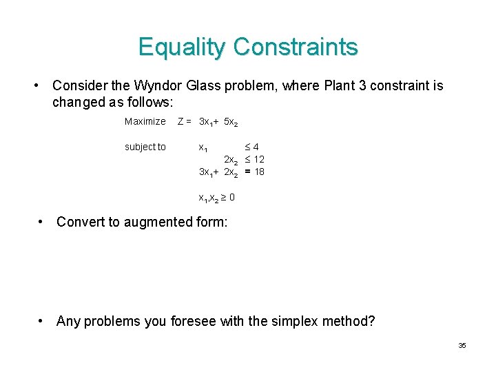
Equality Constraints • Consider the Wyndor Glass problem, where Plant 3 constraint is changed as follows: Maximize subject to Z = 3 x 1+ 5 x 2 x 1 2 x 2 3 x 1+ 2 x 2 4 12 = 18 x 1, x 2 ≥ 0 • Convert to augmented form: • Any problems you foresee with the simplex method? 35

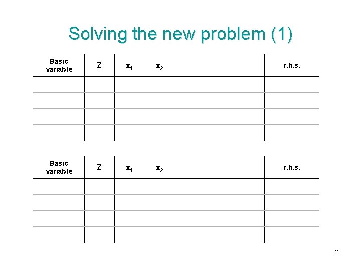
Artificial Variables and the Big M • Introduce artificial variables to the problem • Assign huge penalties in the objective function Maximize subject to Z = 3 x 1+ 5 x 2 x 1 2 x 2 3 x 1+ 2 x 2 4 12 = 18 x 1, x 2 ≥ 0 36

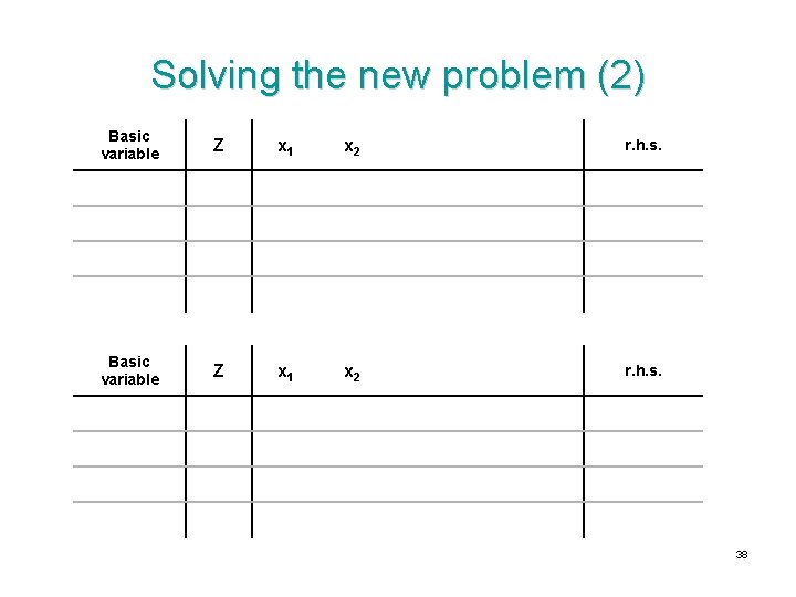
Solving the new problem (1) Basic variable Z x 1 x 2 r. h. s. 37

Solving the new problem (2) Basic variable Z x 1 x 2 r. h. s. 38

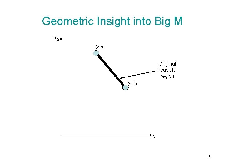
Geometric Insight into Big M x 2 (2, 6) Original feasible region (4, 3) x 1 39

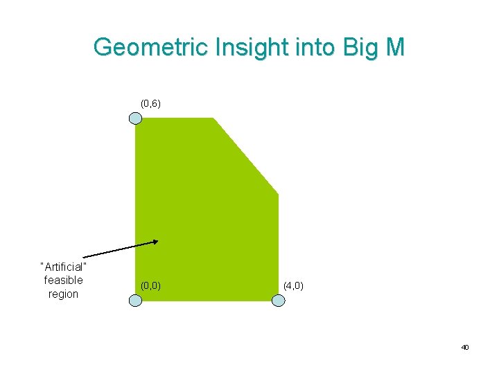
Geometric Insight into Big M (0, 6) “Artificial” feasible region (0, 0) (4, 0) 40

Negative RHS Values • Consider a constraint with bj < 0 – e. g. The number of windows produced should be at most 5 less than the number of doors produced: • Easy fix: • Tough consequences 41

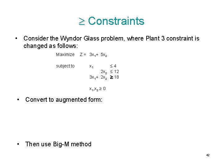
Constraints • Consider the Wyndor Glass problem, where Plant 3 constraint is changed as follows: Maximize subject to Z = 3 x 1+ 5 x 2 x 1 2 x 2 3 x 1+ 2 x 2 4 12 18 x 1, x 2 ≥ 0 • Convert to augmented form: • Then use Big-M method 42

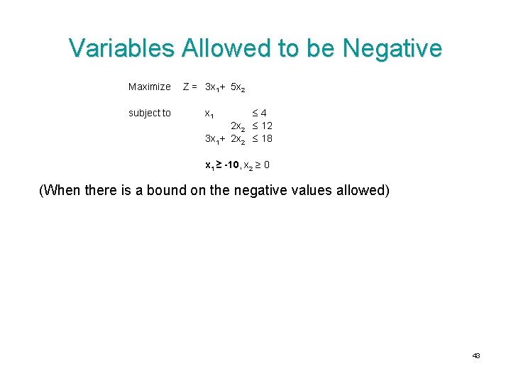
Variables Allowed to be Negative Maximize subject to Z = 3 x 1+ 5 x 2 x 1 2 x 2 3 x 1+ 2 x 2 4 12 18 x 1 ≥ -10, x 2 ≥ 0 (When there is a bound on the negative values allowed) 43

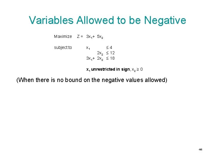
Variables Allowed to be Negative Maximize subject to Z = 3 x 1+ 5 x 2 x 1 2 x 2 3 x 1+ 2 x 2 4 12 18 x 1 unrestricted in sign, x 2 ≥ 0 (When there is no bound on the negative values allowed) 44

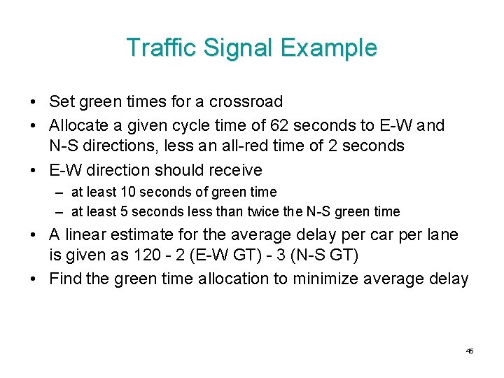
Traffic Signal Example • Set green times for a crossroad • Allocate a given cycle time of 62 seconds to E-W and N-S directions, less an all-red time of 2 seconds • E-W direction should receive – at least 10 seconds of green time – at least 5 seconds less than twice the N-S green time • A linear estimate for the average delay per car per lane is given as 120 - 2 (E-W GT) - 3 (N-S GT) • Find the green time allocation to minimize average delay 45