Solving Linear Programming Models Topics n Computer Solution

Solving Linear Programming Models

Topics n Computer Solution n Sensitivity Analysis

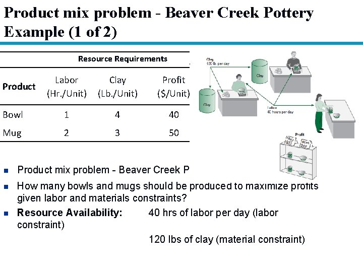
Product mix problem - Beaver Creek Pottery Example (1 of 2) Resource Requirements Labor (Hr. /Unit) Clay (Lb. /Unit) Profit ($/Unit) Bowl 1 4 40 Mug 2 3 50 Product n Product mix problem - Beaver Creek Pottery Company n How many bowls and mugs should be produced to maximize profits given labor and materials constraints? Resource Availability: 40 hrs of labor per day (labor constraint) 120 lbs of clay (material constraint) n

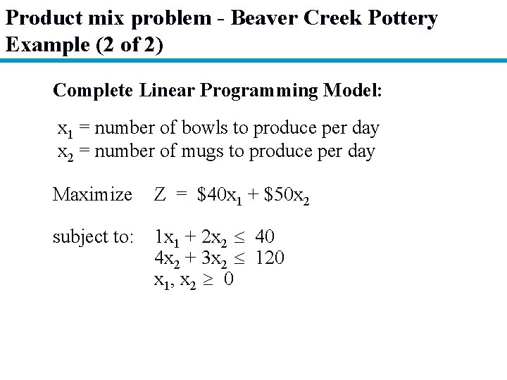
Product mix problem - Beaver Creek Pottery Example (2 of 2) Complete Linear Programming Model: x 1 = number of bowls to produce per day x 2 = number of mugs to produce per day Maximize Z = $40 x 1 + $50 x 2 subject to: 1 x 1 + 2 x 2 40 4 x 2 + 3 x 2 120 x 1, x 2 0

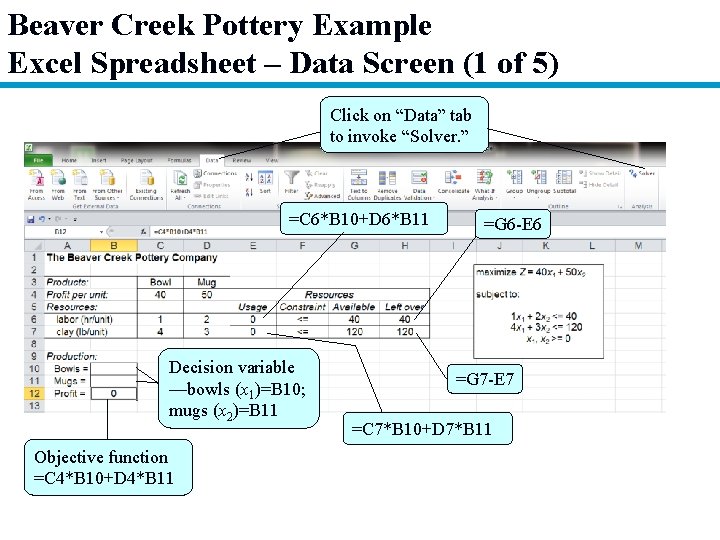
Beaver Creek Pottery Example Excel Spreadsheet – Data Screen (1 of 5) Click on “Data” tab to invoke “Solver. ” =C 6*B 10+D 6*B 11 Decision variable —bowls (x 1)=B 10; mugs (x 2)=B 11 Objective function =C 4*B 10+D 4*B 11 =G 6 -E 6 =G 7 -E 7 =C 7*B 10+D 7*B 11

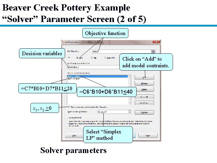
Beaver Creek Pottery Example “Solver” Parameter Screen (2 of 5) Objective function Decision variables =C 7*B 10+D 7*B 11<20 Click on “Add” to add model contraints. =C 6*B 10+D 6*B 11<40 x 1, x 2 >0 Select “Simplex LP” method Solver parameters

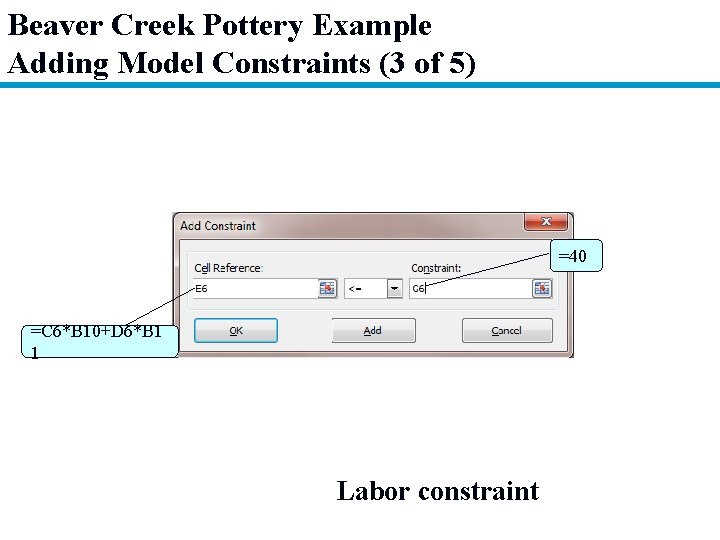
Beaver Creek Pottery Example Adding Model Constraints (3 of 5) =40 =C 6*B 10+D 6*B 1 1 Labor constraint

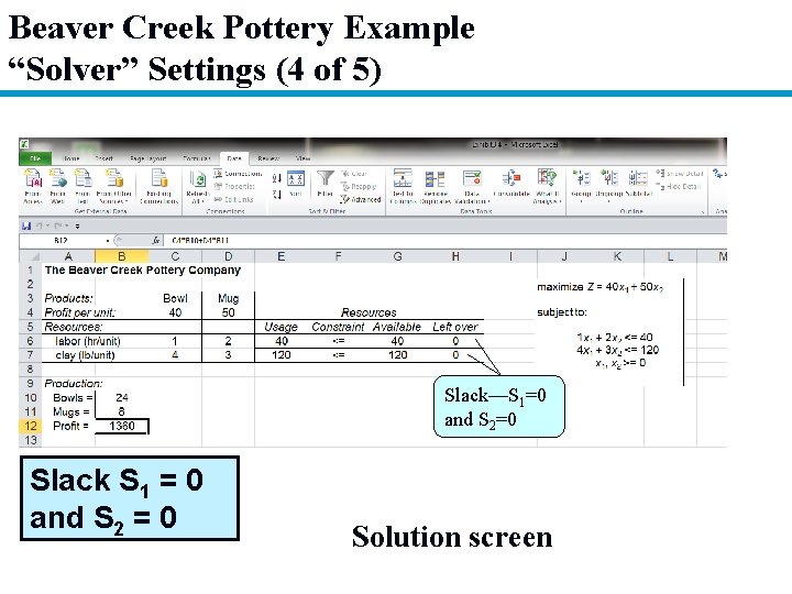
Beaver Creek Pottery Example “Solver” Settings (4 of 5) Slack—S 1=0 and S 2=0 Slack S 1 = 0 and S 2 = 0 Solution screen

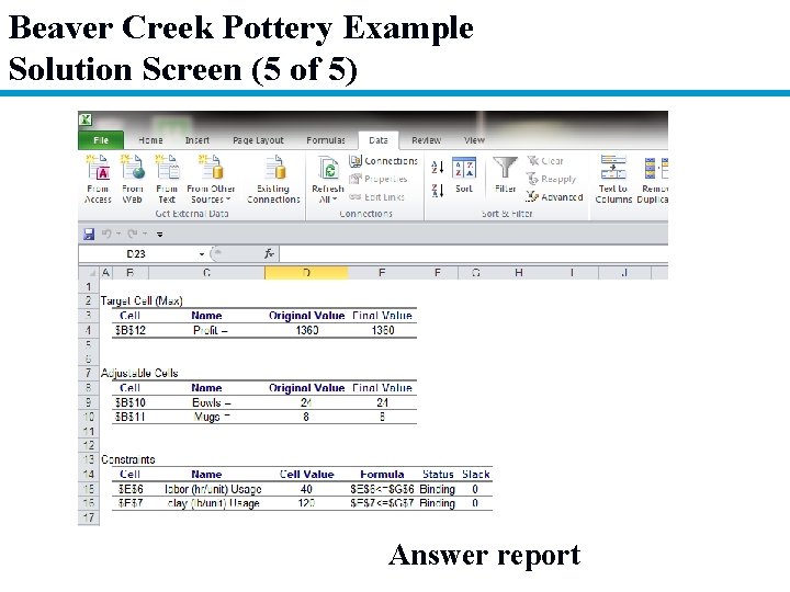
Beaver Creek Pottery Example Solution Screen (5 of 5) Answer report

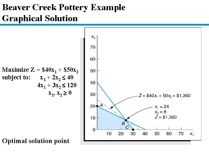
Beaver Creek Pottery Example Graphical Solution Maximize Z = $40 x 1 + $50 x 2 subject to: x 1 + 2 x 2 40 4 x 1 + 3 x 2 120 x 1, x 2 0 Optimal solution point

Sensitivity Analysis n Sensitivity analysis determines the effect on the optimal solution of changes in parameter values of the objective function and constraint equations. n Changes may be reactions to anticipated uncertainties in the parameters or to new or changed information concerning the model.

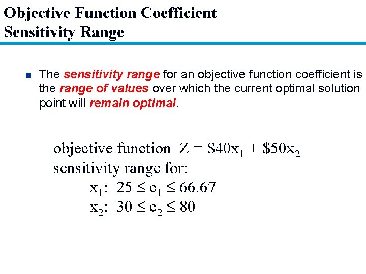
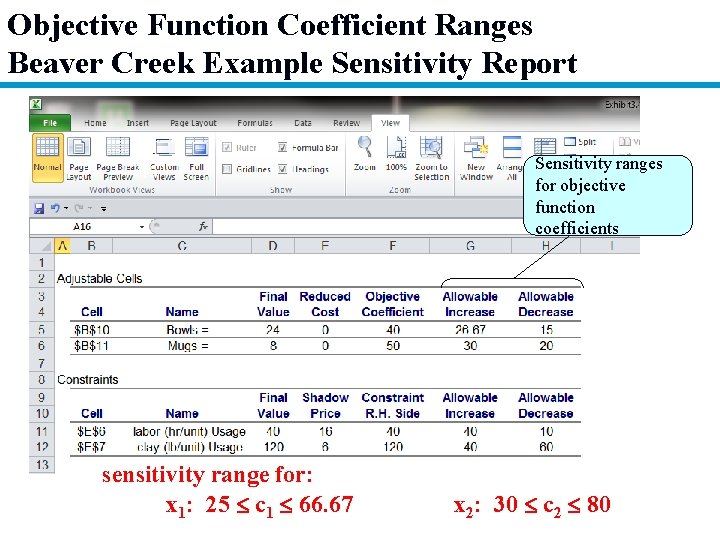
Objective Function Coefficient Sensitivity Range n The sensitivity range for an objective function coefficient is the range of values over which the current optimal solution point will remain optimal. objective function Z = $40 x 1 + $50 x 2 sensitivity range for: x 1: 25 c 1 66. 67 x 2: 30 c 2 80

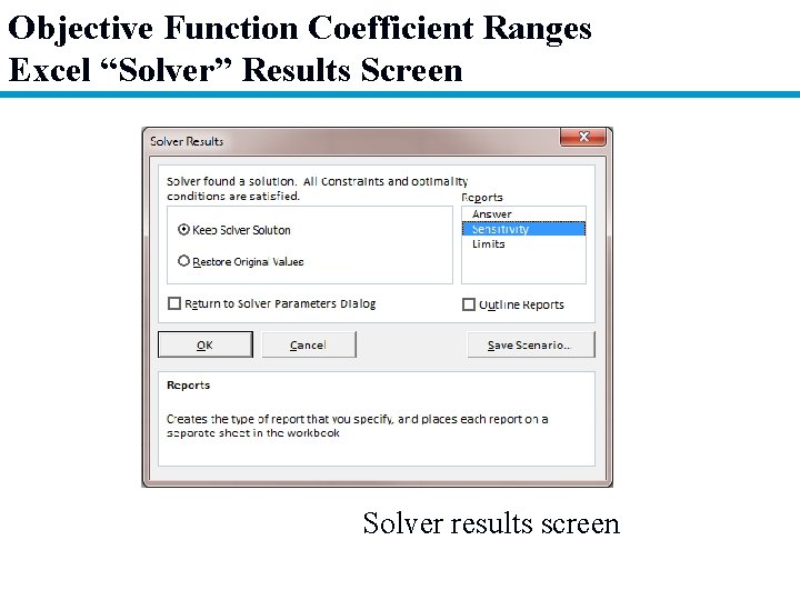
Objective Function Coefficient Ranges Excel “Solver” Results Screen Solver results screen

Objective Function Coefficient Ranges Beaver Creek Example Sensitivity Report Sensitivity ranges for objective function coefficients sensitivity range for: x 1: 25 c 1 66. 67 x 2: 30 c 2 80

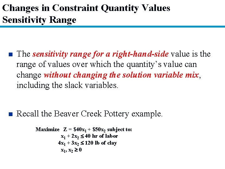
Changes in Constraint Quantity Values Sensitivity Range n The sensitivity range for a right-hand-side value is the range of values over which the quantity’s value can change without changing the solution variable mix, including the slack variables. n Recall the Beaver Creek Pottery example. Maximize Z = $40 x 1 + $50 x 2 subject to: x 1 + 2 x 2 40 hr of labor 4 x 1 + 3 x 2 120 lb of clay x 1, x 2 0

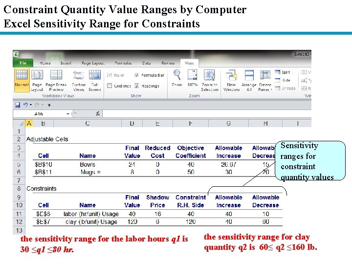
Constraint Quantity Value Ranges by Computer Excel Sensitivity Range for Constraints Sensitivity ranges for constraint quantity values the sensitivity range for the labor hours q 1 is 30 ≤q 1 ≤ 80 hr. the sensitivity range for clay quantity q 2 is 60≤ q 2 ≤ 160 lb.

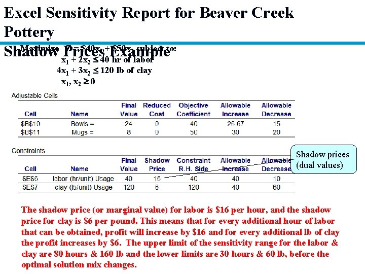
Excel Sensitivity Report for Beaver Creek Pottery Maximize Z = $40 x + $50 x subject to: Shadow Prices Example x + 2 x 40 hr of labor 1 1 2 2 4 x 1 + 3 x 2 120 lb of clay x 1, x 2 0 Shadow prices (dual values) The shadow price (or marginal value) for labor is $16 per hour, and the shadow price for clay is $6 per pound. This means that for every additional hour of labor that can be obtained, profit will increase by $16 and for every additional lb of clay the profit increases by $6. The upper limit of the sensitivity range for the labor & clay are 80 hours & 160 lb and the lower limits are 30 hours & 60 lb, before the optimal solution mix changes.

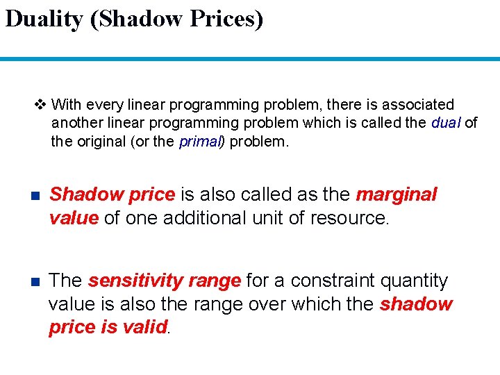
Duality (Shadow Prices) v With every linear programming problem, there is associated another linear programming problem which is called the dual of the original (or the primal) problem. n Shadow price is also called as the marginal value of one additional unit of resource. n The sensitivity range for a constraint quantity value is also the range over which the shadow price is valid.

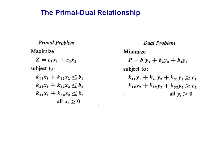
The Primal-Dual Relationship

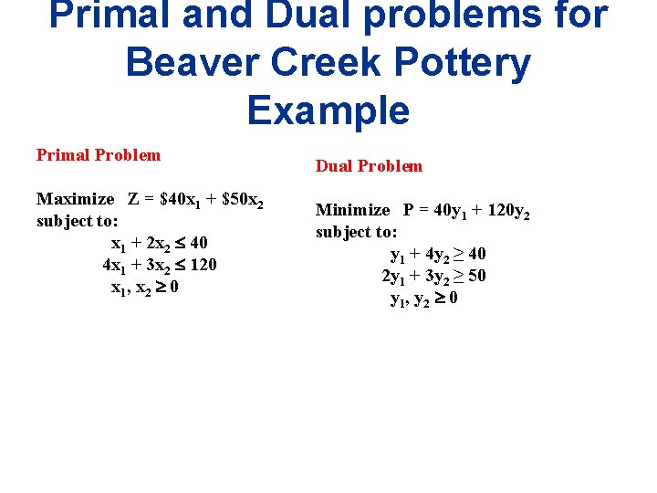
Primal and Dual problems for Beaver Creek Pottery Example Primal Problem Maximize Z = $40 x 1 + $50 x 2 subject to: x 1 + 2 x 2 40 4 x 1 + 3 x 2 120 x 1, x 2 0 Dual Problem Minimize P = 40 y 1 + 120 y 2 subject to: y 1 + 4 y 2 ≥ 40 2 y 1 + 3 y 2 ≥ 50 y 1, y 2 0

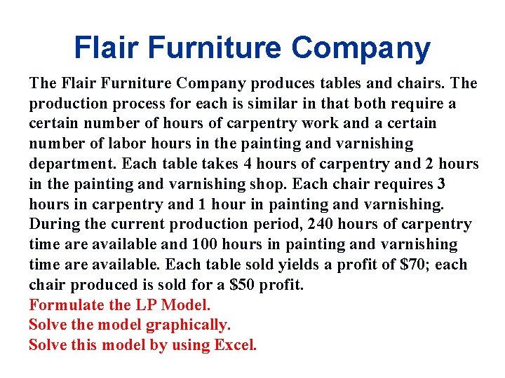
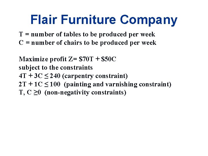
Flair Furniture Company The Flair Furniture Company produces tables and chairs. The production process for each is similar in that both require a certain number of hours of carpentry work and a certain number of labor hours in the painting and varnishing department. Each table takes 4 hours of carpentry and 2 hours in the painting and varnishing shop. Each chair requires 3 hours in carpentry and 1 hour in painting and varnishing. During the current production period, 240 hours of carpentry time are available and 100 hours in painting and varnishing time are available. Each table sold yields a profit of $70; each chair produced is sold for a $50 profit. Formulate the LP Model. Solve the model graphically. Solve this model by using Excel.

Flair Furniture Company T = number of tables to be produced per week C = number of chairs to be produced per week Maximize profit Z= $70 T + $50 C subject to the constraints 4 T + 3 C ≤ 240 (carpentry constraint) 2 T + 1 C ≤ 100 (painting and varnishing constraint) T, C ≥ 0 (non-negativity constraints)

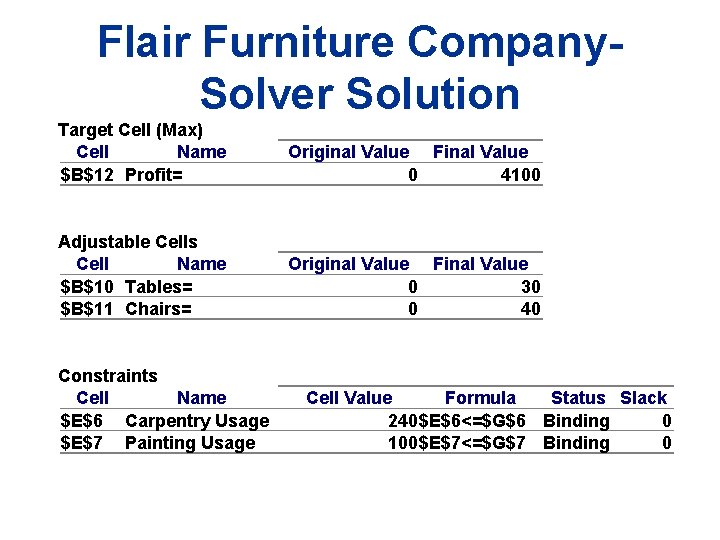
Flair Furniture Company. Solver Solution Target Cell (Max) Cell Name $B$12 Profit= Original Value Final Value 0 4100 Adjustable Cells Cell Name $B$10 Tables= $B$11 Chairs= Original Value Final Value 0 30 0 40 Constraints Cell Name $E$6 Carpentry Usage $E$7 Painting Usage Cell Value Formula Status Slack 240$E$6<=$G$6 Binding 0 100$E$7<=$G$7 Binding 0

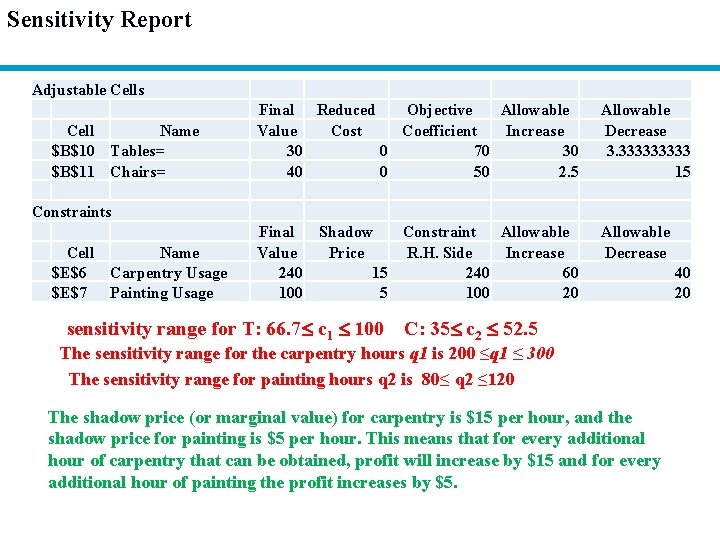
Sensitivity Report Adjustable Cells Cell Name $B$10 Tables= $B$11 Chairs= Final Reduced Objective Allowable Value Cost Coefficient Increase 30 0 70 30 40 0 50 2. 5 Allowable Decrease 3. 33333 15 Constraints Cell Name $E$6 Carpentry Usage $E$7 Painting Usage Final Value 240 100 Allowable Decrease Shadow Constraint Allowable Price R. H. Side Increase 15 240 60 5 100 20 sensitivity range for T: 66. 7 c 1 100 C: 35 c 2 52. 5 The sensitivity range for the carpentry hours q 1 is 200 ≤q 1 ≤ 300 The sensitivity range for painting hours q 2 is 80≤ q 2 ≤ 120 The shadow price (or marginal value) for carpentry is $15 per hour, and the shadow price for painting is $5 per hour. This means that for every additional hour of carpentry that can be obtained, profit will increase by $15 and for every additional hour of painting the profit increases by $5. 40 20

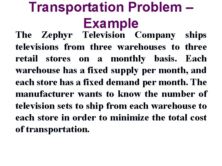
Transportation Problem – Example The Zephyr Television Company ships televisions from three warehouses to three retail stores on a monthly basis. Each warehouse has a fixed supply per month, and each store has a fixed demand per month. The manufacturer wants to know the number of television sets to ship from each warehouse to each store in order to minimize the total cost of transportation.

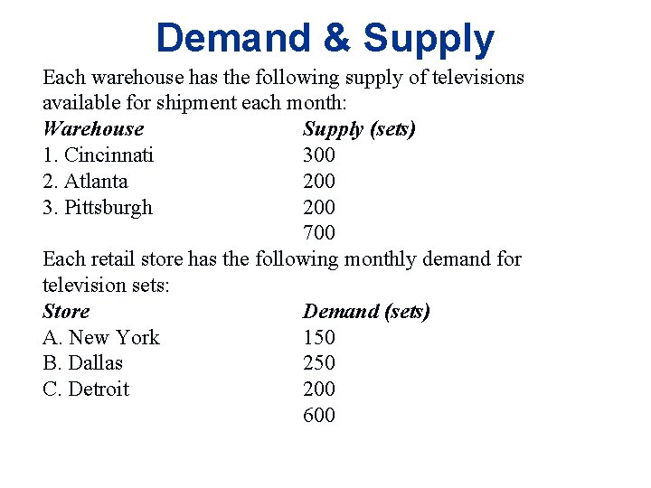
Demand & Supply Each warehouse has the following supply of televisions available for shipment each month: Warehouse Supply (sets) 1. Cincinnati 300 2. Atlanta 200 3. Pittsburgh 200 700 Each retail store has the following monthly demand for television sets: Store Demand (sets) A. New York 150 B. Dallas 250 C. Detroit 200 600

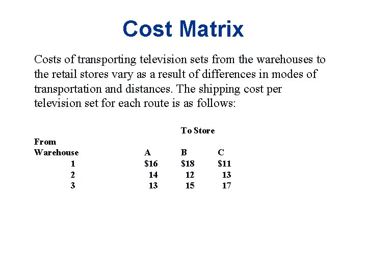
Cost Matrix Costs of transporting television sets from the warehouses to the retail stores vary as a result of differences in modes of transportation and distances. The shipping cost per television set for each route is as follows: To Store From Warehouse 1 2 3 A $16 14 13 B $18 12 15 C $11 13 17

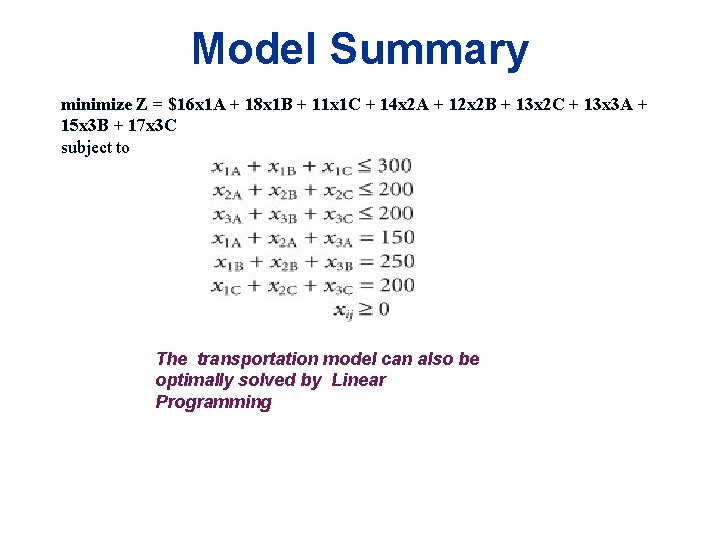
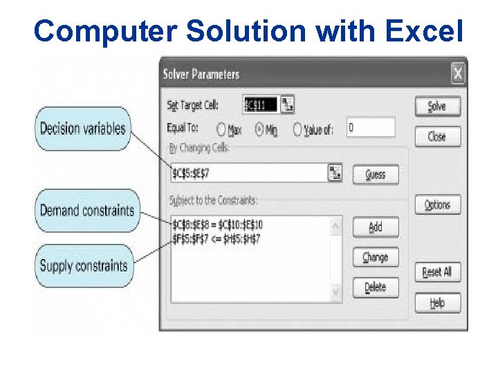
Model Summary minimize Z = $16 x 1 A + 18 x 1 B + 11 x 1 C + 14 x 2 A + 12 x 2 B + 13 x 2 C + 13 x 3 A + 15 x 3 B + 17 x 3 C subject to The transportation model can also be optimally solved by Linear Programming

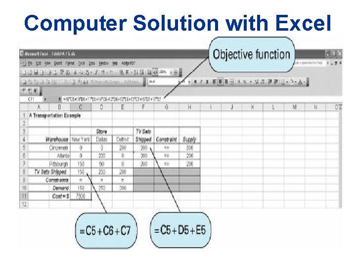
Computer Solution with Excel

Computer Solution with Excel

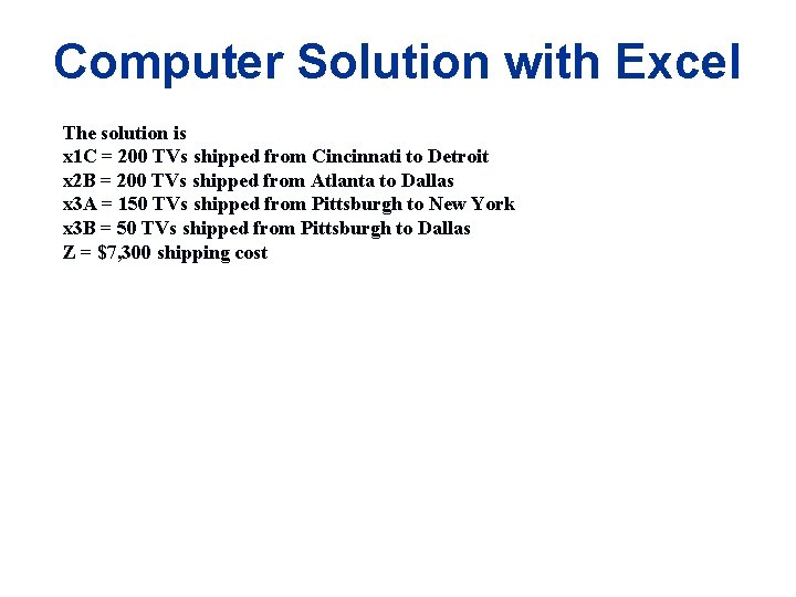
Computer Solution with Excel The solution is x 1 C = 200 TVs shipped from Cincinnati to Detroit x 2 B = 200 TVs shipped from Atlanta to Dallas x 3 A = 150 TVs shipped from Pittsburgh to New York x 3 B = 50 TVs shipped from Pittsburgh to Dallas Z = $7, 300 shipping cost