Solvation Models Solvent Effects Many reactions take place

Solvent Effects • Many reactions take place in solution • Short-range effects • Typically

Solvation Models • Some describe explicit solvent molecules • Some treat solvent as a

Solvation Methods in Molecular Simulations explicit solvent • Explicit Solvent vs. Implicit Solvent Explicit:

Two Kinds of Solvatin Models Explicit solvent models Continuum solvation models Features All solvent

Explicit QM Water Models • Sometimes as few as 3 explicit water molecules can

Explicit Hybrid Solvation Model Red = highest level of theory (MP 2, CISDT) Blue

Continuum (Reaction Field) Models • Consider solvent as a uniform polarizable medium of fixed

Self-Consistent Reaction Field • Solvent: A uniform polarizable medium with a dielectric constant e

Models Differ in 5 Aspects 1. Size and shape of the solute cavity 2.

Solute Cavity Size and Shape Spherical (Born) (Kirkwood) Ellipsoidal (Onsager) van de Waals r

The Cavity • Simple models Sphere Ellipsoid • Molecular shaped models Van der Waals

Description of Solute M Solute molecule M may be described by: – classical molecular

Describing the Dielectric Medium • Usually taken to be a homogeneous static medium of

Why Implicit Solvent? Method Pros Cons Explicit Solvent (all-atom description) Implicit Solvent (Continuum description)

Slides: 27

Download presentation

Solvation Models

Solvent Effects • Many reactions take place in solution • Short-range effects • Typically concentrated in the first solvation sphere • Examples: H-bonds, preferential orientation near an ion • Long-range effects • Polarization (charge screening)

Solvation Models • Some describe explicit solvent molecules • Some treat solvent as a continuum • Some are hybrids of the above two: – Treat first solvation sphere explicitly while treating surrounding solvent by a continuum model – These usually treat inner solvation shell quantum mechanically, outer solvation shell classically Each of these models can be further subdivided according to theory involved: classical (MM) or quantum mechanical

Solvation Methods in Molecular Simulations explicit solvent • Explicit Solvent vs. Implicit Solvent Explicit: considering the molecular details of each solvent molecules Implicit: treating the solvent as a continuous medium (Reaction Field Method) implicit solvent

Two Kinds of Solvatin Models Explicit solvent models Continuum solvation models Features All solvent molecules are explicitly represented. Respresent solvent as a continuous medium. Advantages Detail information is Simple, inexpensive to provided. Generally more calculate accurate. Disadvantages Expensive for computation Ignore specific short-range effects. Less accurate.

Explicit QM Water Models • Sometimes as few as 3 explicit water molecules can be used to model a reaction adequately: Could use HF, DFT, MP 2, CISD(T) or other theory.

Explicit Hybrid Solvation Model Red = highest level of theory (MP 2, CISDT) Blue = intermed. level of theory (HF, AM 1, PM 3) Black = lowest level of theory (MM 2, MMFF), or Continuum

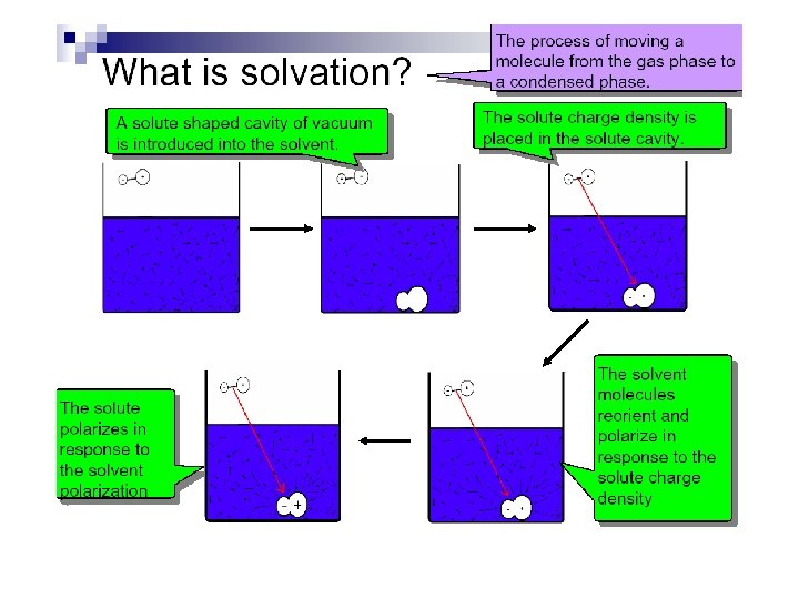
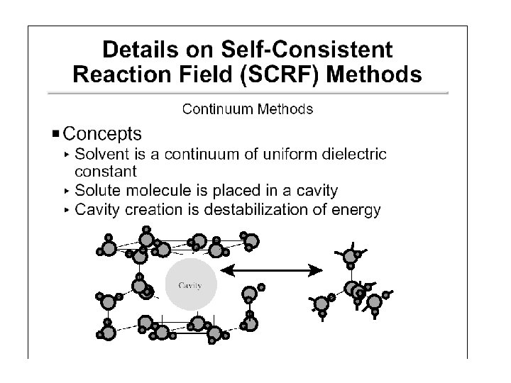
Continuum (Reaction Field) Models • Consider solvent as a uniform polarizable medium of fixed dielectric constant e having a solute molecule M placed in a suitably shaped cavity. e

Self-Consistent Reaction Field • Solvent: A uniform polarizable medium with a dielectric constant e • Solute: A molecule in a suitably shaped cavity in the medium • Solvation free energy: DGsolv = DGcav + DGdisp + DGelec M 1. Create a cavity in the medium costs energy (destabilization). e 2. Dispersion (mainly Van der Waals) interactions between solute and solvent lower the energy (stabilization). 3. Polarization between solute and solvent induces charge redistribution until self-consistent and lowers the energy (stabilization).

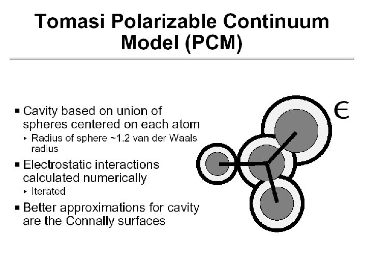
Models Differ in 5 Aspects 1. Size and shape of the solute cavity 2. Method of calculating the cavity creation and the dispersion contributions 3. How the charge distribution of solute M is represented 4. Whether the solute M is described classically or quantum mechanically 5. How the dielectric medium is described. (these 5 aspects will be considered in turn on the following slides)

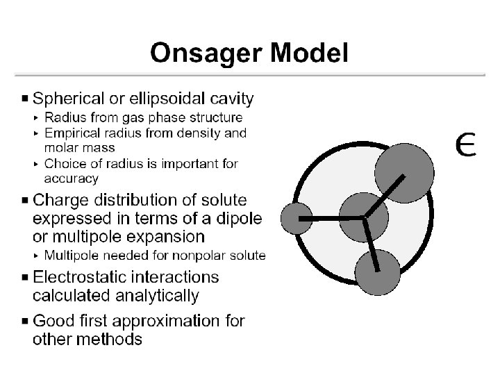
Solute Cavity Size and Shape Spherical (Born) (Kirkwood) Ellipsoidal (Onsager) van de Waals r r

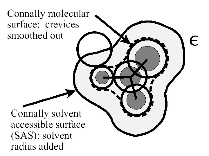
The Cavity • Simple models Sphere Ellipsoid • Molecular shaped models Van der Waals surface Not accessible to solvent Solvent accessible surface Determined by QM wave function and/or electron density

Description of Solute M Solute molecule M may be described by: – classical molecular mechanics (MM) – semi-empirical quantum mechanics (SEQM), – ab initio quantum mechanics (QM) – density functional theory (DFT), or – post Hartree-Fock electron correlation methods (MP 2 or CISDT).

Describing the Dielectric Medium • Usually taken to be a homogeneous static medium of constant dielectric constant e • May be allowed to have a dependence on the distance from the solute molecule M. • In some models, such as those used to model dynamic processes, the dielectric may depend on the rate of the process (e. g. , the response of the solvent is different for a “fast” process such as an electronic excitation than for a “slow” process such as a molecular rearrangement. )

Why Implicit Solvent? Method Pros Cons Explicit Solvent (all-atom description) Implicit Solvent (Continuum description) • Full details on the molecular structures • Realistic physical picture of the system • No explicit solvent atoms • Treatment of solute at highest level possible (QM) • Many atoms--> expensive • Long runs required to equilibrate solvent to solute • Often solvent and solute are not polarizable. • Large fluctuations due to use of small system size • Need to define an artificial boundary between the solute and solvent • No “good” model for treating short range effects (dispersion and cavity)