Solutions of Autonomous Linear Systems SOLUTION State transition

Solutions of Autonomous Linear Systems SOLUTION: State transition matrix describes how states evolve. Properties of the State Transition Matrix 1 -

2 - 3 - State transition matrix satisfies the matrix differential equation with initial condition.

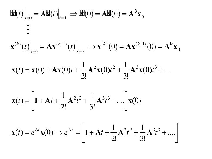
Solutions of Non-autonomous Linear Systems Assumption: Substituting the solution in one gets

For linear time-invariant systems One should calculate in order to find the solution.

How to calculate 1 - Using its definition as a series Taylor series expansion of at ? : Reminder

How to calculate ? 2 - Jordan Canonical Form By a similarity transformation, the matrix A can be upper-diagonalized. For an eigenvalue with (algebraic) multiplicity there are Jordan blocks. and it is called the geometric multiplicity. It is the number of independent eigenvectors that can be found using. Other (generalized) eigenvectors will be found using.

Columns of P are the. . . . . How can we find ?

Find using Jordan canonical form!

>> A=[0 0 0 1; 2 1 -1 -1 0 -1; 0 0 2 1 0 0; 0 0 0 2 0 0; 0 0 2 0; -1 0 0 2 ] A = 0 0 0 1 2 1 -1 0 0 2 1 0 0 0 0 0 2 0 -1 0 0 2 >> [P, J]=jordan(A) P = 0 0 0 2 -1 0 2 -3 -2 0 1 0 0 0 0 1 0 0 0 2 1 0 J = 2 1 0 0 0 2 0 0 0 1 1 0 0 0 0 0 1 0 0 0 2 >> expm(J*t) ans = [ exp(2*t), t*exp(2*t), 0, 0, 0] [ 0, 0, exp(t), t*exp(t), (t^2*exp(t))/2, 0] [ 0, 0, exp(t), t*exp(t), 0] [ 0, 0, 0, 0, exp(2*t )] >> pretty(ans)

3 - Laplace Transform Definition: Let be a continuous or piecewise continuous function. If then the Laplace transform of is given by Pierre-Simon, marquis de Laplace 1749 -1827 is the Laplace transform of . is the inverse Laplace transform.

Properties of the Laplace Transform 1 - Uniqueness Proof will be skipped. . 2 - Linearity If Proof: , are real constants, then

3 - Proof:

4 - Proof:

5 - Proof:

6 - Proof:

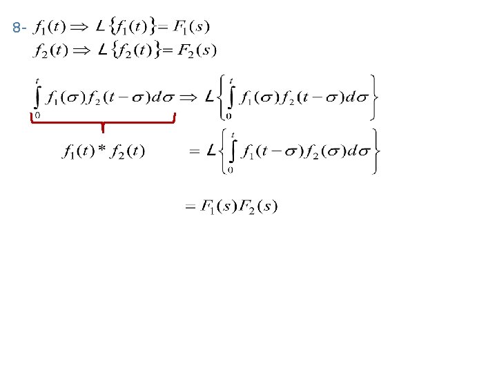
7 - Proof:

Some usefull formulas for Laplace Transform: http: //en. wikipedia. org/wiki/Laplace_transform

Finding the Zero-Input Solution using Laplace Transform zero-input solution

Find the zero-input solution!

How can one find the output invariant systems. input system impulse response for a given input output for linear time-

Finding the Zero-State Solution using Laplace Transform 0 zero-state solution

Finding the Total Solution using Laplace Transform OUTPUT

Find the output for the given LTI system.