Solution of Nonlinear Equation Dr Asaf Varol avarolmix

Solution of Nonlinear Equation Dr. Asaf Varol avarol@mix. wvu. edu 1

Introduction • Solutions to algebraic, differential, and integral equations relating certain physical parameters for a given problem • Algebraic equations divided into two categories: (1) Linear and (2) Nonlinear • Linear: an equation which contains the first power of the unknown, explicitly or implicitly, indicating a linear variation of the unknown parameter as a function of the other known parameters. • Example: distance, s, traveled by an object which was originally at a location s = s 0 at time t = 0, and moving at constant speed, v, is related to time by s = s 0 + vt • which is a linear relationship between s and v , and also between s and t since v is assumed not changing with time. 2

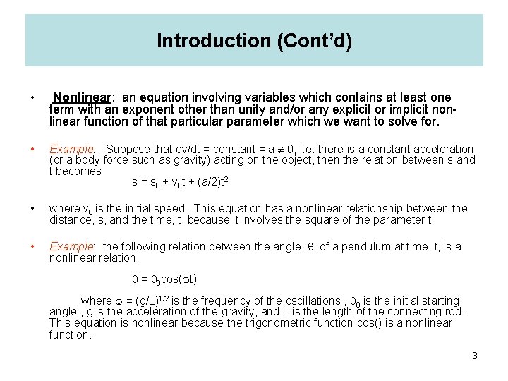
Introduction (Cont’d) • Nonlinear: an equation involving variables which contains at least one term with an exponent other than unity and/or any explicit or implicit nonlinear function of that particular parameter which we want to solve for. • Example: Suppose that dv/dt = constant = a 0, i. e. there is a constant acceleration (or a body force such as gravity) acting on the object, then the relation between s and t becomes s = s 0 + v 0 t + (a/2)t 2 • where v 0 is the initial speed. This equation has a nonlinear relationship between the distance, s, and the time, t, because it involves the square of the parameter t. • Example: the following relation between the angle, , of a pendulum at time, t, is a nonlinear relation. = 0 cos( t) where = (g/L)1/2 is the frequency of the oscillations , 0 is the initial starting angle , g is the acceleration of the gravity, and L is the length of the connecting rod. This equation is nonlinear because the trigonometric function cos() is a nonlinear function. 3

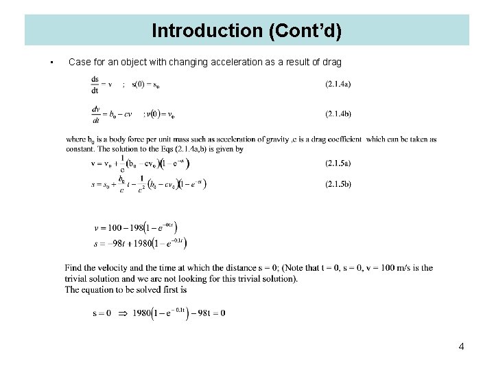
Introduction (Cont’d) • Case for an object with changing acceleration as a result of drag 4

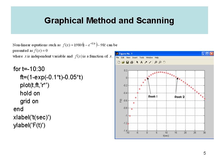
Graphical Method and Scanning for t=-10: 30 ft=(1 -exp(-0. 1*t)-0. 05*t) plot(t, ft, 'r*') hold on grid on end xlabel('t(sec)') ylabel('F(t)') 5

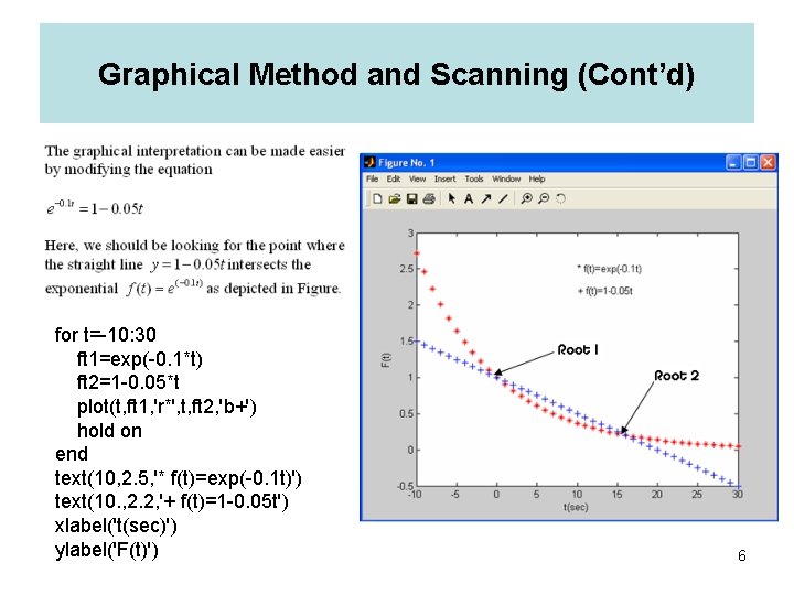
Graphical Method and Scanning (Cont’d) for t=-10: 30 ft 1=exp(-0. 1*t) ft 2=1 -0. 05*t plot(t, ft 1, 'r*', t, ft 2, 'b+') hold on end text(10, 2. 5, '* f(t)=exp(-0. 1 t)') text(10. , 2. 2, '+ f(t)=1 -0. 05 t') xlabel('t(sec)') ylabel('F(t)') 6

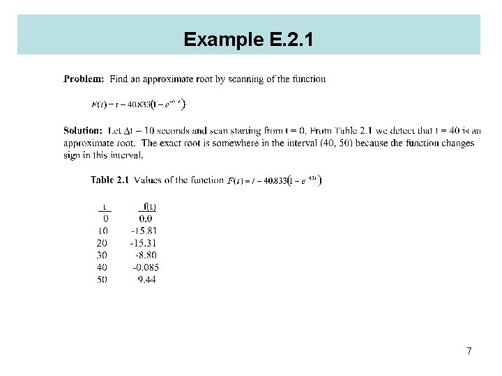
Example E. 2. 1 7

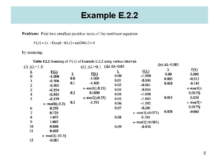
Example E. 2. 2 8

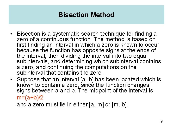
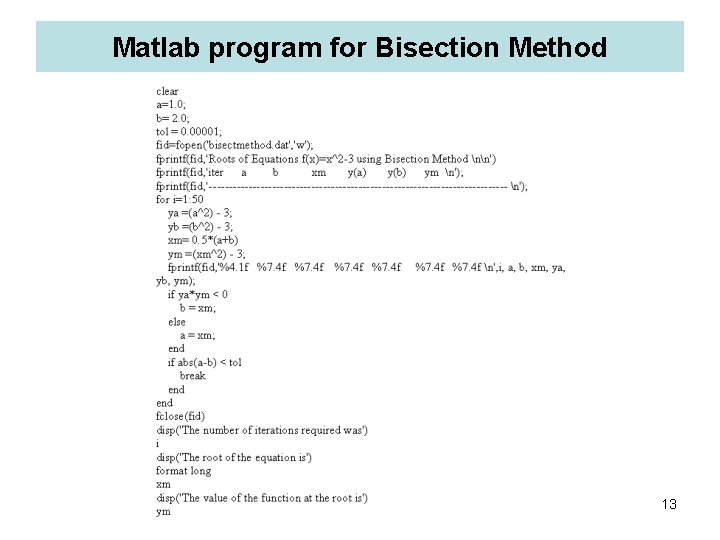
Bisection Method • Bisection is a systematic search technique for finding a zero of a continuous function. The method is based on first finding an interval in which a zero is known to occur because the function has opposite signs at the ends of the interval, then dividing the interval into two equal subintervals, and determining which subinterval contains a zero, and continuing the computations on the subinterval that contains the zero. • Suppose that an interval [a, b] has been located which is known to contain a zero, since the function changes signs between a and b. The midpoint of the interval is m=(a+b)/2 and a zero must lie in either [a, m] or [m, b]. 9

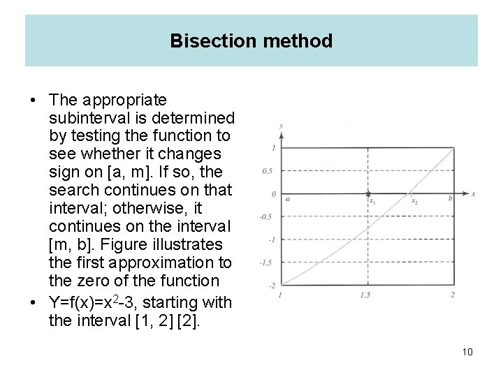
Bisection method • The appropriate subinterval is determined by testing the function to see whether it changes sign on [a, m]. If so, the search continues on that interval; otherwise, it continues on the interval [m, b]. Figure illustrates the first approximation to the zero of the function • Y=f(x)=x 2 -3, starting with the interval [1, 2] [2]. 10

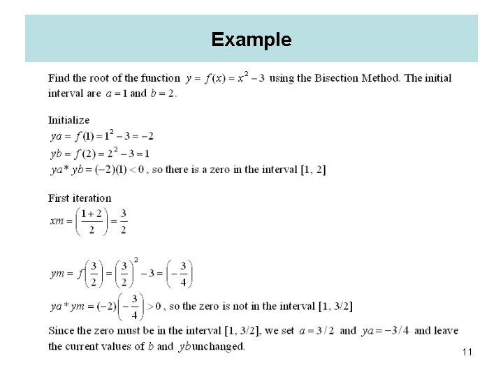
Example 11

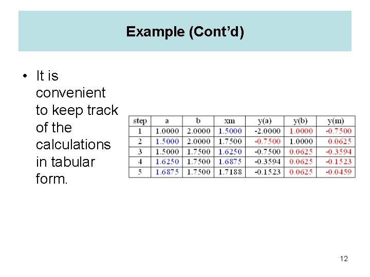
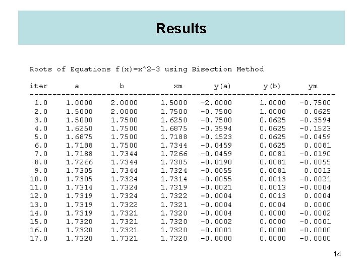
Example (Cont’d) • It is convenient to keep track of the calculations in tabular form. 12

Matlab program for Bisection Method 13

Results 14

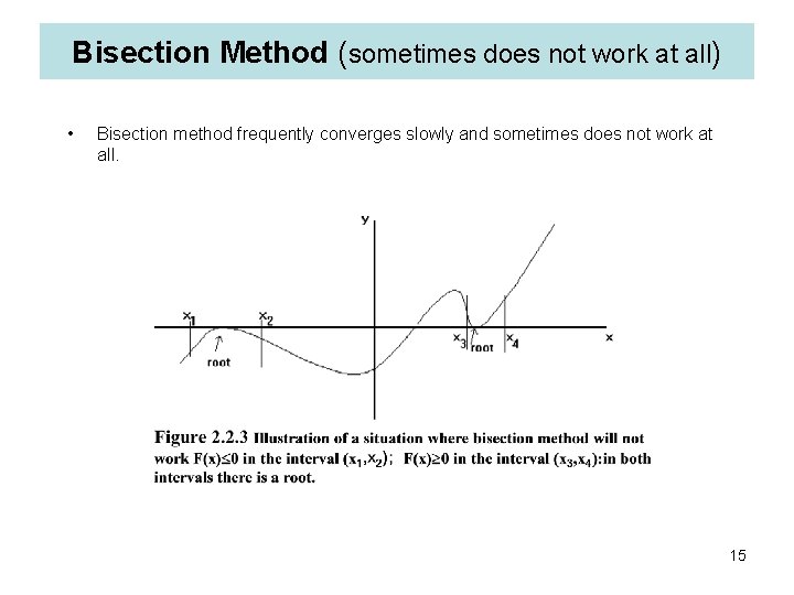
Bisection Method (sometimes does not work at all) • Bisection method frequently converges slowly and sometimes does not work at all. 15

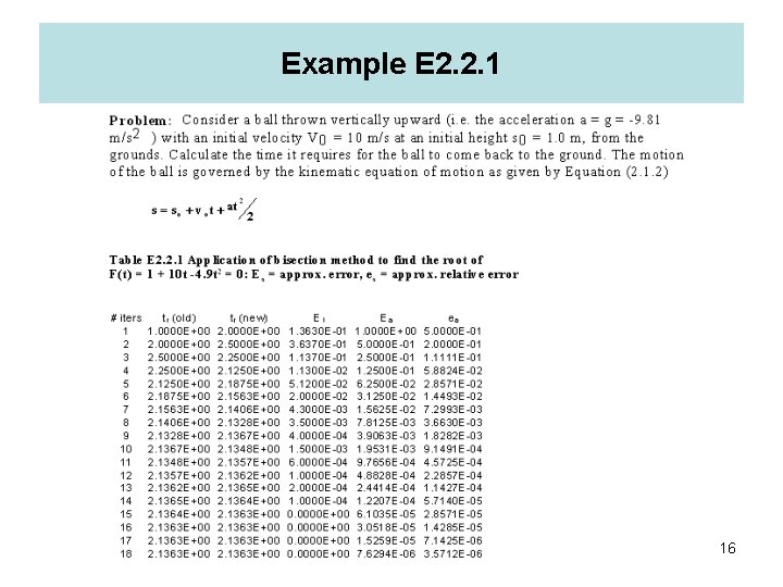
Example E 2. 2. 1 16

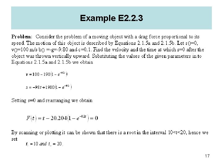
Example E 2. 2. 3 17

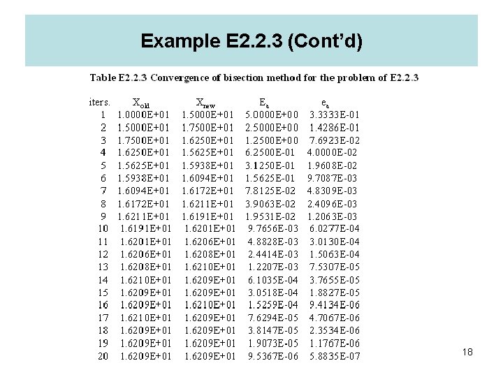
Example E 2. 2. 3 (Cont’d) 18

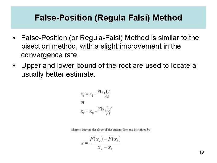
False-Position (Regula Falsi) Method • False-Position (or Regula-Falsi) Method is similar to the bisection method, with a slight improvement in the convergence rate. • Upper and lower bound of the root are used to locate a usually better estimate. 19

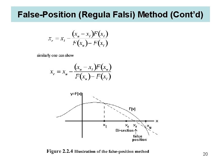
False-Position (Regula Falsi) Method (Cont’d) 20

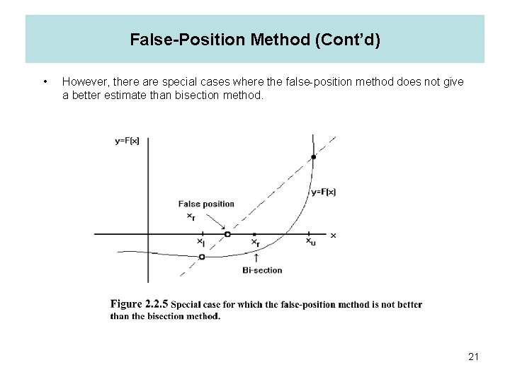
False-Position Method (Cont’d) • However, there are special cases where the false-position method does not give a better estimate than bisection method. 21

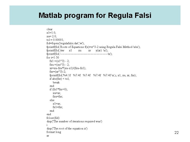
Matlab program for Regula Falsi 22

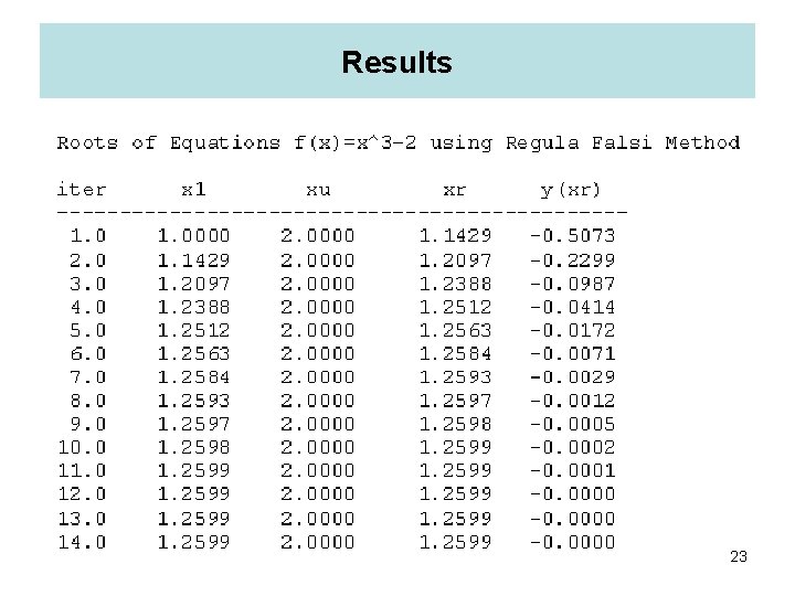
Results 23

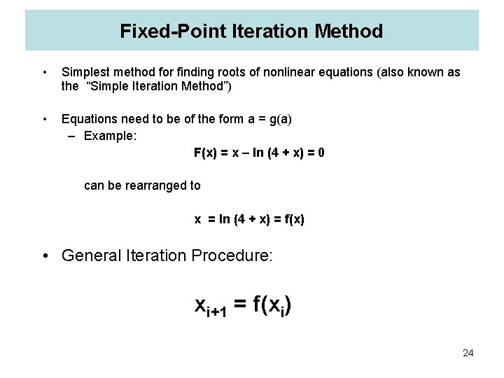
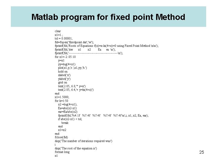
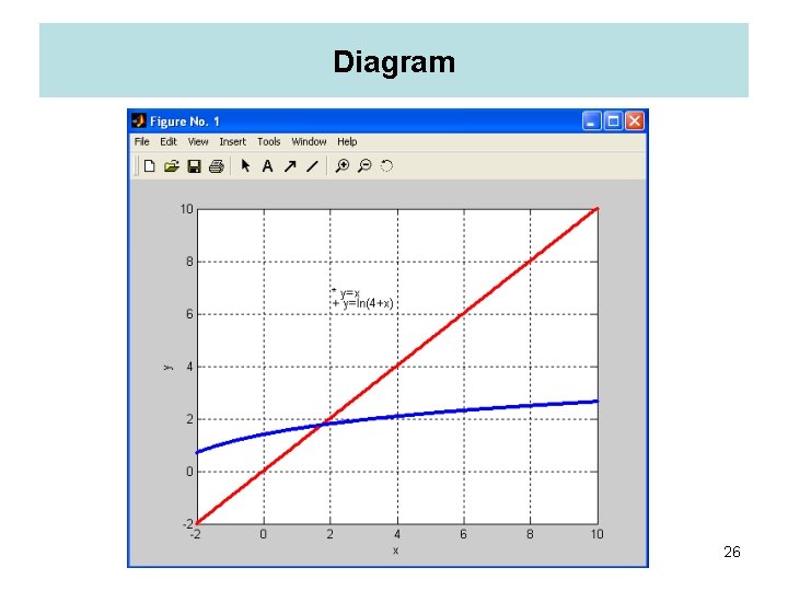
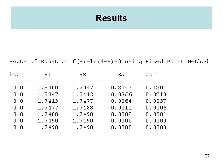
Fixed-Point Iteration Method • Simplest method for finding roots of nonlinear equations (also known as the “Simple Iteration Method”) • Equations need to be of the form a = g(a) – Example: F(x) = x – ln (4 + x) = 0 can be rearranged to x = ln (4 + x) = f(x) • General Iteration Procedure: xi+1 = f(xi) 24

Matlab program for fixed point Method 25

Diagram 26

Results 27

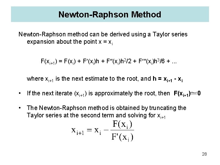
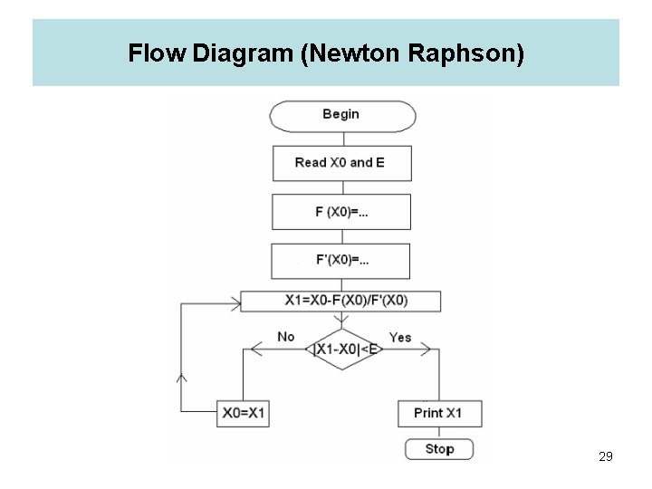
Newton-Raphson Method Newton-Raphson method can be derived using a Taylor series expansion about the point x = xi F(xi+1) = F(xi) + F (xi)h 2/2 + F (xi)h 3/6 +. . . where xi+1 is the next estimate to the root, and h = xi+1 - xi • If the next iterate (xi+1) is approximately the root, then F(xi+1) 0 • The Newton-Raphson method is obtained by truncating the Taylor series at the second term and solving for xi+1 28

Flow Diagram (Newton Raphson) 29

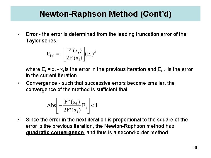
Newton-Raphson Method (Cont’d) • • • Error - the error is determined from the leading truncation error of the Taylor series. where Ei = xr - xi is the error in the previous iteration and Ei+1 is the error in the current iteration Convergence - such that successive errors become smaller, the convergence of the method is sufficient that Since the error in the next iteration is proportional to the square of the error is the previous iteration, the Newton-Raphson method has quadratic convergence, and thus is a second-order method 30

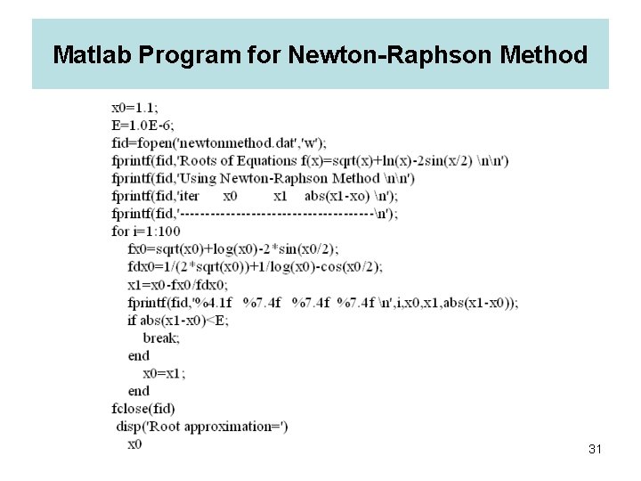
Matlab Program for Newton-Raphson Method 31

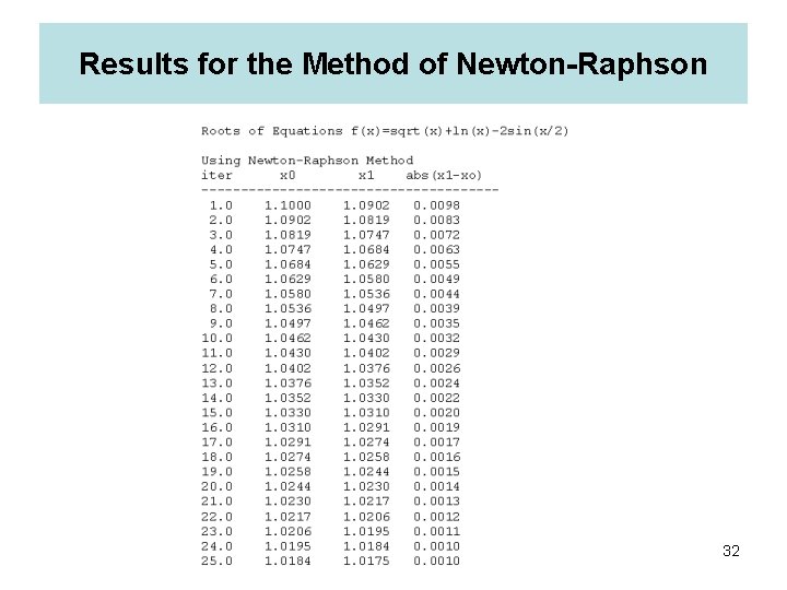
Results for the Method of Newton-Raphson 32

• End of Chapter 2 a 33

References • • • Celik, Ismail, B. , “Introductory Numerical Methods for Engineering Applications”, Ararat Books & Publishing, LCC. , Morgantown, 2001 Fausett, Laurene, V. “Numerical Methods, Algorithms and Applications”, Prentice Hall, 2003 by Pearson Education, Inc. , Upper Saddle River, NJ 07458 Rao, Singiresu, S. , “Applied Numerical Methods for Engineers and Scientists, 2002 Prentice Hall, Upper Saddle River, NJ 07458 Mathews, John, H. ; Fink, Kurtis, D. , “Numerical Methods Using MATLAB” Fourth Edition, 2004 Prentice Hall, Upper Saddle River, NJ 07458 Varol, A. , “Sayisal Analiz (Numerical Analysis), in Turkish, Course notes, Firat University, 2001 34