Solar Modulation Heliosphere In the heliopshere there is


 equation: Flux J = p")


= Archimedean Spiral")


![P(q) Initial Energy []Ge. V Prop Time [Days] Proton Propagation Kinetic Energy [Ge. V]](https://slidetodoc.com/presentation_image_h2/b062250df428e9f12a3c4e58bd8291c6/image-22.jpg "P(q) Initial Energy []Ge. V Prop Time [Days] Proton Propagation Kinetic Energy [Ge. V]")

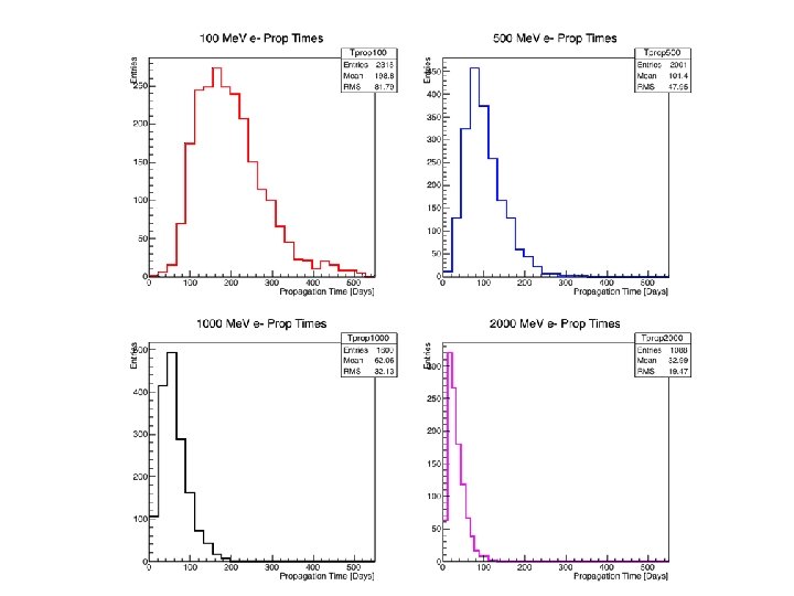
![Kinetic Energy [Ge. V] P(q) Initial Energy []Ge. V Prop Time [Days] Electron Propagation](https://slidetodoc.com/presentation_image_h2/b062250df428e9f12a3c4e58bd8291c6/image-24.jpg "Kinetic Energy [Ge. V] P(q) Initial Energy []Ge. V Prop Time [Days] Electron Propagation")

![Antiprotons & positrons Flux (m sr s Gev)-1 pbar Kinetic Energy [Ge. V]](https://slidetodoc.com/presentation_image_h2/b062250df428e9f12a3c4e58bd8291c6/image-27.jpg "Antiprotons & positrons Flux (m sr s Gev)-1 pbar Kinetic Energy [Ge. V]")

- Slides: 28
Solar Modulation Heliosphere In the heliopshere there is a variable supersonic solar wind with an embedded a “frozen-in” turbulent magnetic field. This leads to global and temporal variations in the intensity of CR as a function of position inside the heliosphere. This process is identified as the solar modulation of CR A void in the local interstellar medium where Sun B field dominates Modulation plays a role in galactic CR flux up to 30 Ge. V Fundamental to deconvolve the LIS spectrum at low energy, ie spectra at Earth location below 30 Ge. V are NOT representative of the LIS spectrum
Low Energy Cosmic Rays Not representative of LIS spectrum 2
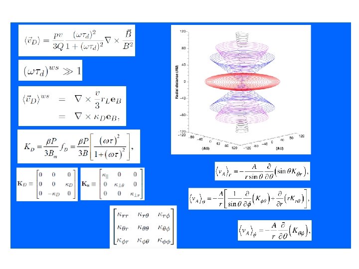
Propagation in the heliosphere is decribed by Parker (1965) equation: Flux J = p 2 f Diffusion Small Scale Magnetic Field irregolarity Convection Drift Presence of the solar wind moving out from the Sun Large Scale structure of magnetic field (gradients&curvature) Energetic Loss Due to adiabatic expansion of the solar wind
• Diffusion is anisotropic along the parallel and perpendicular directions wrt the local B field • Needed three diffusion coefficients • They depend on the turbulence scale of the IMF • Described by QLT of turbulence
Effective diffusion tensor =
Model of Propagation No local sources Q = 0 Stationary ∂/∂t=0 2 D with axial symmetry ∂/∂F=0
SOLARPROP • Numerical integration is made by using the Stochastic Differential Equation approach with backward time integration in the framework of solarprop • Solarprop is a package (Kappl, Comp. Sc. , 2015) publicly available at XXXX • Very flexible, upgradable and user-friendly package • Original program modified for: • Some physics bugs corrected: • b = R/E instead of b = p/E • Drift speeds ~p instead of ~R • Angle for Neutral Drift Speed effects corrected • Parker Magnetic Field with polar corrections used • Parallel and perpendicular diffusion coefficients with breaks in rigidity implemented • Polar enhancement of tranverse perpendicular diffusion coeff Kqq • Latitude- and tilt angle- dependent solar wind speed with termination shock
Parker Equation Ito’s lemma, see e. g. Gardiner, 1985 Stochastic Differential Equations 8
Magnetic Field tg(y)= Archimedean Spiral
Field polarity A Configuration for A>0 Configuration for A<0
Solar Activity A>0 A<0 A>0 The solar activity is related to: - Sunspot number (<10 minimum; >100 maximum) - Wavy Neutral Sheet opening/tilt angle (10° minimum ; >75° maximum) A<0
Wavy Neutral Sheet Solar Wind and Magnetic Field Latitudinal Dependence B=0
Solar Wind Low Solar Activity High Solar Activity • Different speed latitudinal profiles depending on the solar cycle phase • No defined polarity A during high solar activity at maximum
R = 50 AU R = 10 AU R = 5 AU R = 1 AU Parker Field + Jopikii&Kota Mod Ideal Parker Field With VSW = 400 kms-1
R = 50 AU R = 10 AU R = 5 AU R = 1 AU With VSW = 400 kms-1 tg(y)= Modified Geometry (Smith&Bieber, 1991) Ideal Parker Field Spiral Angle
Diffusion coefficents A Fnr. K|| Fnq. K|| Fnr= Fnq = 0. 02 as default
Model of solar wind speed latitudinal dependence Termination Shock compression ratio S = 2. 5 TS scale length L = 1. 2 AU TS position r. TS = 90 AU V 0 = 400 km/s Tilt Angle < 15° Solar Min 15° <Tilt Angle < 40° Tilt Angle > 40° Solar Max Potgieter et al. , 2015
Solar Wind Speed Radial Dependence r. TS High Latitude Low Latitude Termination Shock compression ratio S = 2. 5 TS scale length L = 1. 2 AU TS position r. TS = 90 AU V 0 = 400 km/s
LEAP 87 He ATIC AMS 01 BESS Polar II NO tilt angle data BESS Polar I SMILI I, MASS 89 NB: tensione fra i dati di smili e mass SMILI II, MASS 91
Pamela 2007/7, A>0 Proton Modulation Pamela 2009/7, A>0 Bess 1997/7 A<0. Min Bess 1998/8 A<0 Bess 1999/8 A<0 Bess 2000/8 A<0, Max
P(q) Initial Energy []Ge. V Prop Time [Days] Proton Propagation Kinetic Energy [Ge. V] DE/E Kinetic Energy [Ge. V] Entrance Latitude [Deg] 2009 Polarity A >0 Kinetic Energy [Ge. V] Prop Time [Days]
Electron modulation
Kinetic Energy [Ge. V] P(q) Initial Energy []Ge. V Prop Time [Days] Electron Propagation DE/E Kinetic Energy [Ge. V] Entrance Latitude [Deg] Kinetic Energy [Ge. V] Prop Time [Days] 2009 Polarity A>0
Helium Modulation He modulation using the proton model parameters Bess Polar 2007/12
Antiprotons & positrons Flux (m sr s Gev)-1 pbar Kinetic Energy [Ge. V]
Goals • Set up a realistic global modulation model to describe the propagation of CR in the heliosphere • Time lag for e- and He • Compare modulation in A<0 and A>0 periods for all the particles o Charge dependence of modulation o Role of diffusion and drifts at min and max solar activity o Use BESS, PAMELA and AMS 02 data • Compare unusual minimum of cycle 24 to the previous one • Study modulation of light ions (Li, Be, B, C, …) • Make the model fully 3 d Many different LIS spectra around We are using milan group public LIS Spectra We need the most up-to-dated LIS spectra NO e+ reliable LIS spectrum