Software Testing and Reliability and Risk Assessment Aditya

Software Testing and Reliability and Risk Assessment Aditya P. Mathur Purdue University August 12 -16 @ Guidant Corporation Minneapolis/St Paul, MN Graduate Assistants: Ramkumar Natarajan Baskar Sridharan Last update: August 16, 2002 Software Reliability Copyright Aditya P. Mathur

Reliability and risk assessment n Learning objectives 1 . What is software reliability? 2 . How to estimate software reliability? 3 . What is risk assessment? 4 . How to estimate risk using application architecture? Software Testing and Reliability © Aditya P. Mathur 2002 2

References 1 . Statistical Methods in Software Engineering: Reliability and Risk, Nozer D. Singpurwalla and Simon P. Wilson, Springer, 1999. 2 . Software Reliability, Measurement, Prediction, Application, John D. Musa, Anthony Iannino, and Kazuhira Okumoto, Mc. Graw-Hill Book Company, 1987. 3 . A Methodology for Architecture Level Reliability Risk Analysis, S. M. Yacoub and H. H. Ammar, IEEE Transactions on Software Engineering, June 2002, V 28, N 6, pp 529 -547. 4 . Real-Time UML: Developing Efficient Objects for Embedded Systems. Bruce Powell Douglass, Addison. Wesley, 1998. Software Testing and Reliability © Aditya P. Mathur 2002 3

Software Reliability n n Software reliability is the probability of failure free operation of an application in a specified operating environment and time period. Reliability is one quality metric. Others include performance, maintainability, portability, and interoperability Software Testing and Reliability © Aditya P. Mathur 2002 4

Operating Environment n Hardware: Machine and configuration n Software: OS, libraries, etc. n Usage (Operational profile) Software Testing and Reliability © Aditya P. Mathur 2002 5

Uncertainty n n n Uncertainty is a common phenomena in our daily lives. In software engineering, uncertainty occurs in all phases of the software life cycle. Examples: • Will the schedule be met? • How many months will it take to complete the design? • How many testers to deploy? • What is the number of faults remaining faults? Software Testing and Reliability © Aditya P. Mathur 2002 6

Probability and statistics n n n Uncertainty can be quantified and managed using probability theory and statistical inference. Probability theory assists with quantification and combination of uncertainties. Statistical inference assists with revision of uncertainties in light of the available data. Software Testing and Reliability © Aditya P. Mathur 2002 7

Probability Theory n n In any software process there are known and unknown quantities. The known quantities constitute history and is denoted by H. The unknown quantities are referred to as random quantities. Each unknown quantity is denoted by a capital letter such as T or X. Software Testing and Reliability © Aditya P. Mathur 2002 8

Random Variables n n n Specific values of T and X are denoted by lower case letters t and x and are known as realizations of the corresponding random quantities. When a random quantity can assume numerical values it is known as a random variable. Example: If X denotes the outcome of a coin toss, then X can assume a value 0 (for head) and 1 (for tail). X is a random variable under the assumption that on each toss the outcome is not known with certainty. Software Testing and Reliability © Aditya P. Mathur 2002 9

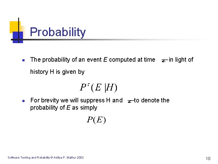
Probability n The probability of an event E computed at time in light of history H is given by n For brevity we will suppress H and probability of E as simply Software Testing and Reliability © Aditya P. Mathur 2002 to denote the 10

Random Events n n A random quantity that may assume one of two values, say e 1 and e 2, is a random event often denoted by E. Examples: • Program P will fail on the next run. • Application A contains no errors. • The time to next failure of application A will be greater than t. • The design for application A will be completed in less than 3 months. Software Testing and Reliability © Aditya P. Mathur 2002 11

Binary Random Variables n n When e 1 and e 2 are numerical values, such as 0 and 1, then E is known as a binary random variable. A discrete random variable is one whose realizations are countable. n n Example: Number of failures encountered over four hours of application use. A continuous random variable is one whose realizations are not countable. n Example: Time to next failure. Software Testing and Reliability © Aditya P. Mathur 2002 12

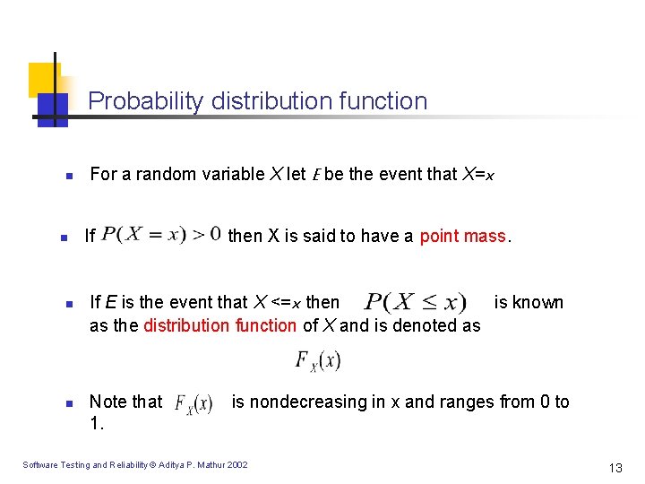
Probability distribution function n n For a random variable X let E be the event that X=x If then X is said to have a point mass. If E is the event that X <=x then is known as the distribution function of X and is denoted as Note that 1. is nondecreasing in x and ranges from 0 to Software Testing and Reliability © Aditya P. Mathur 2002 13

Probability density function n If X is continuous and takes all values in some interval I and is differentiable with respect to x for all x in I , then is absolutely continuous. The derivative of at x is denoted by known as the probability density function of X. and is dx is the approximate probability that the random variable X takes on a value in the interval x and x+dx. Software Testing and Reliability © Aditya P. Mathur 2002 14

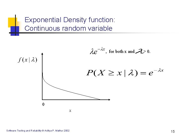
Exponential Density function: Continuous random variable , for both x and > 0. 0 x Software Testing and Reliability © Aditya P. Mathur 2002 15

Binomial Distribution n n Suppose that an application is executed N times each with a distinct input. We want to know the number of inputs, X, on which the application will fail. Note that the proportion of the correct outputs is a measure of the reliability of the application. X can assume values x =0, 1, 2, …, N. We are interested in the probability that X=x. Each input to the application can be assumed to be a Bernoulli trial. This gives us Bernoulli random variables Xi, i=1, 2, …, N. Each Xi is a 1 if the application fails and 0 otherwise. Note that X= X 1+X 2+…+XN. Software Testing and Reliability © Aditya P. Mathur 2002 16

Binomial Distribution [contd. ] Under certain assumptions, the following probability model, known as the Binomial distribution, is used. n n Here p is the probability that Xi = 1 for i=1, …, N. In other words, p is the probability of failure of any single run. Software Testing and Reliability © Aditya P. Mathur 2002 17

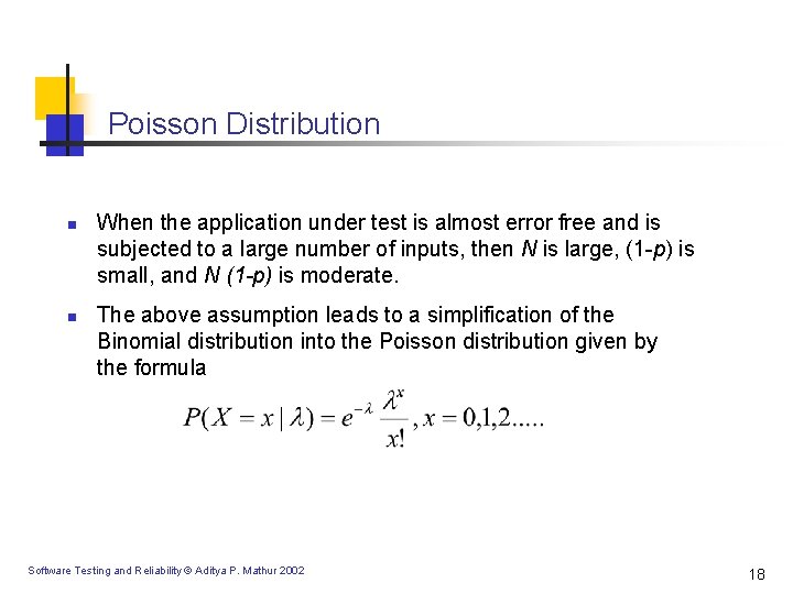
Poisson Distribution n n When the application under test is almost error free and is subjected to a large number of inputs, then N is large, (1 -p) is small, and N (1 -p) is moderate. The above assumption leads to a simplification of the Binomial distribution into the Poisson distribution given by the formula Software Testing and Reliability © Aditya P. Mathur 2002 18

Software Reliability: Types n n n Reliability on a single execution: P(X=1|H), modeled by Bernoulli distribution. Reliability over N executions: P(X=x|H), for x=0, 1, 2, …N, given by Binomial distribution or Poisson distribution for large N and small parameter value p. Reliability over an infinite number of executions: P(X=x|H), for x=1, 2, …N. Note that we are interested in the number of inputs after which the first failure occurs. This is given by geometric distribution. Software Testing and Reliability © Aditya P. Mathur 2002 19

Software Reliability: Types [contd. ] n n n When the inputs to software occur continuously over time, then we are interested in P(X>=x|H), i. e. the probability that the first failure occurs after x time units. This is given by the exponential distribution. The time of occurrence to the kth failure can be given by the Gamma distribution. There are several other models of reliability, over one hundred! Software Testing and Reliability © Aditya P. Mathur 2002 20

Software failures: Sources of uncertainty Uncertainty about the presence and location of defects. Uncertainty about the use of run types. Will a run for a given input state cause a failure? Software Testing and Reliability © Aditya P. Mathur 2002 21

Failure Process n Inputs arrive at an application at random times. n Some inputs cause failures and others do not. n n T 1, T 2, …denote (CPU) times between application failures. Most reliability models are centered around the interfailure times. Software Testing and Reliability © Aditya P. Mathur 2002 22

Failure Intensity and Reliability n n Failure intensity is the number of failures experienced within a unit of time. For example, the failure intensity of an application might be 0. 3 failures/hr. Failure intensity is an alternate way of expressing reliability, R( ), which is the probability of no failures over time duration . For a constant failure intensity we have R( )=e- . It is safe to assume that during testing and debugging, the failure intensity decreases with time and thus the reliability increases. Software Testing and Reliability © Aditya P. Mathur 2002 23

Jelinski and Moranda Model [1972] n n n The application contains an unknown number N of defects. Each time the application fails the defect that caused the failure is removed. Debugging is perfect. Constant relationship between the number of defects and the failure rate. Ti is proportional to (N-I+1). Software Testing and Reliability © Aditya P. Mathur 2002 24

Jelinski and Moranda Model [contd. ] n Thus, given 0=S 0<=S 1<=…. <=Si, i=1, 2… and some constant c, we obtain the following failure intensity, where S 0, S 1, …, Si are supposed software failure times, failure rate r. Ti is given by: for Note that the failure rate drops by a constant amount. S 0=0 S 1 Software Testing and Reliability © Aditya P. Mathur 2002 S 3 time t 25

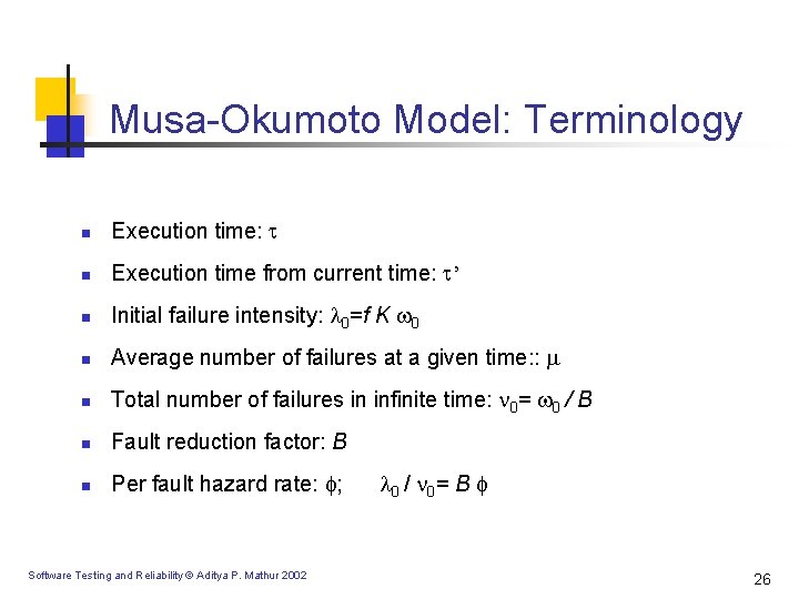
Musa-Okumoto Model: Terminology n Execution time: n Execution time from current time: ’ n Initial failure intensity: 0=f K 0 n Average number of failures at a given time: : n Total number of failures in infinite time: 0= 0 / B n Fault reduction factor: B n Per fault hazard rate: ; Software Testing and Reliability © Aditya P. Mathur 2002 0 / 0 = B 26

Musa-Okumoto Model: Terminology [contd. ] n Number of inherent faults: 0= I I n Number of inherent faults per source instructions: I n Fault exposure ratio: K n Number of source instructions: I n Instruction execution rate: r n Executable object instructions: I n Linear execution frequency: f=r/I Software Testing and Reliability © Aditya P. Mathur 2002 27

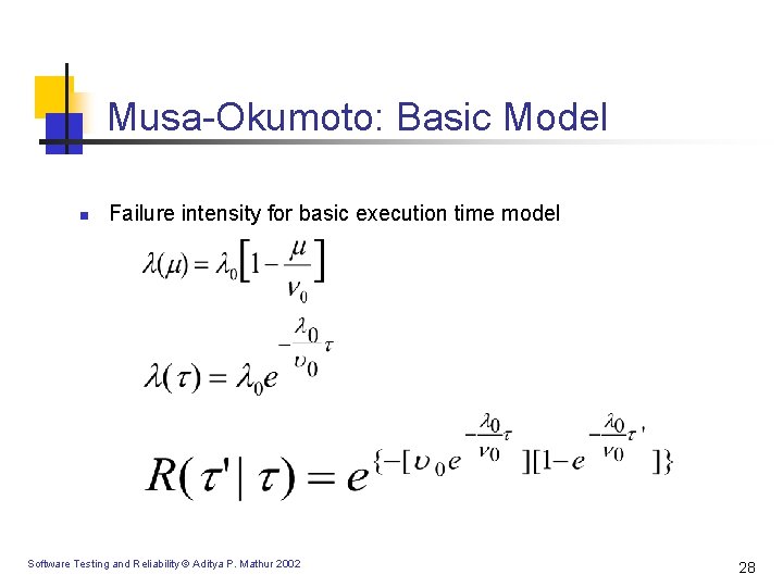
Musa-Okumoto: Basic Model n Failure intensity for basic execution time model Software Testing and Reliability © Aditya P. Mathur 2002 28

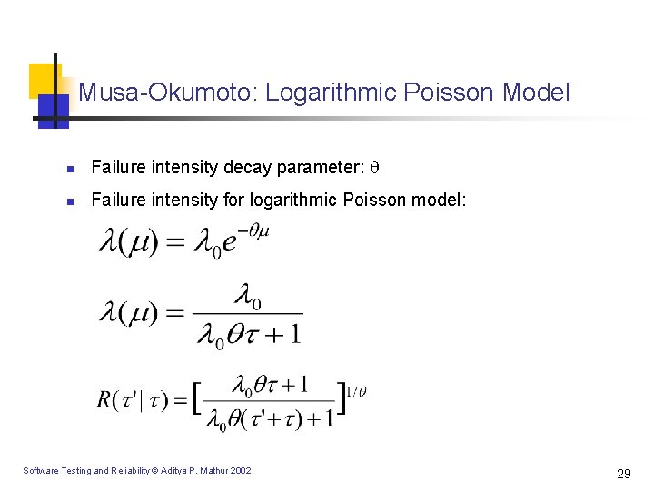
Musa-Okumoto: Logarithmic Poisson Model n Failure intensity decay parameter: n Failure intensity for logarithmic Poisson model: Software Testing and Reliability © Aditya P. Mathur 2002 29

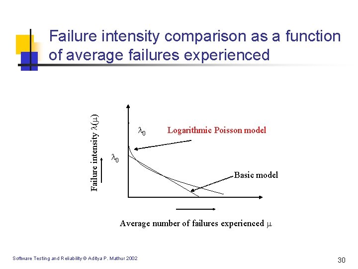
Failure intensity ( ) Failure intensity comparison as a function of average failures experienced 0 Logarithmic Poisson model 0 Basic model Average number of failures experienced Software Testing and Reliability © Aditya P. Mathur 2002 30

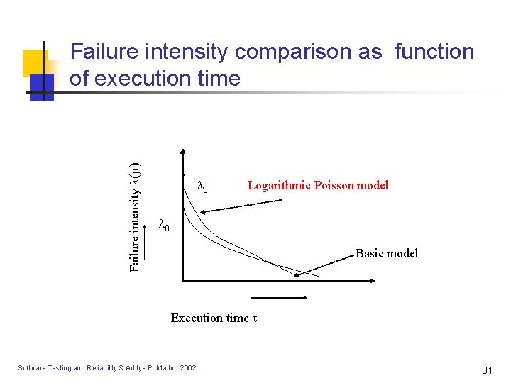
Failure intensity ( ) Failure intensity comparison as function of execution time 0 Logarithmic Poisson model 0 Basic model Execution time Software Testing and Reliability © Aditya P. Mathur 2002 31

Which Model to use? n n Uniform operational profile: Use the basic model Non-uniform operational profile: Use the logarithmic Poisson model Software Testing and Reliability © Aditya P. Mathur 2002 32

Other issues n Counting failures n When is a defect repaired n Impact of imperfect repair Software Testing and Reliability © Aditya P. Mathur 2002 33

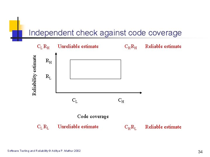
Independent check against code coverage Reliability estimate CL RH Unreliable estimate CH RH Reliable estimate CH RL Reliable estimate RH RL CL CH Code coverage CL RL Unreliable estimate Software Testing and Reliability © Aditya P. Mathur 2002 34

Operational Profile n n n A quantitative characterization of how an application will be used. This characterization requires a knowledge of input variables. Input state is a vector of values of all input variables. Input variables: An interrupt is an input variable and so are all environment variables and variables whose values are input by the user via the keyboard or from a file in response to a prompt. Internal variables, computed from one or more input variables are not input variables. Intermediate results and interrupts generated during the execution as a result of the execution should not be considered as input variables. n n Software Testing and Reliability © Aditya P. Mathur 2002 35

Operational Profile [contd. ] n n Runs of an application that begin with identical input states belong to the same run type. Example 1: Two withdrawals from the same person from the same account and of the same dollar amount. Example 2: Reservations made for two different people on the same flight belong to different run types. Function: Grouping of different run types. A function is conceived at the time of requirements analysis. Software Testing and Reliability © Aditya P. Mathur 2002 36

Operational Profile [contd. ] n n Function: A set of different run types. A function is conceived at the time of requirements analysis. A function is analogous to a use-case. Operation: A set of run types for the application that is built. Software Testing and Reliability © Aditya P. Mathur 2002 37

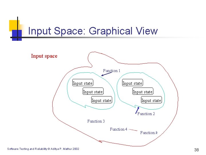
Input Space: Graphical View Input space Function 1 Input state Input state Function 2 Function 3 Function 4 Software Testing and Reliability © Aditya P. Mathur 2002 Function k 38

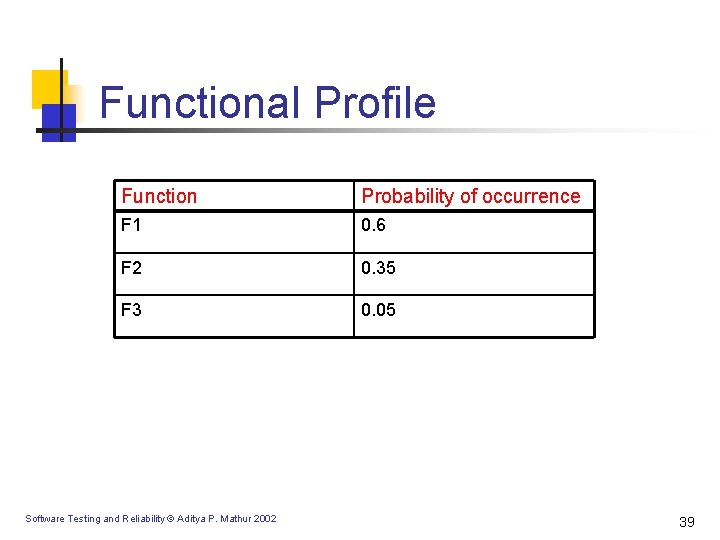
Functional Profile Function Probability of occurrence F 1 0. 6 F 2 0. 35 F 3 0. 05 Software Testing and Reliability © Aditya P. Mathur 2002 39

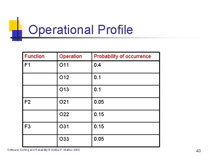
Operational Profile Function Operation Probability of occurrence F 1 O 11 0. 4 O 12 0. 1 O 13 0. 1 O 21 0. 05 O 22 0. 15 O 31 0. 15 O 33 0. 05 F 2 F 3 Software Testing and Reliability © Aditya P. Mathur 2002 40

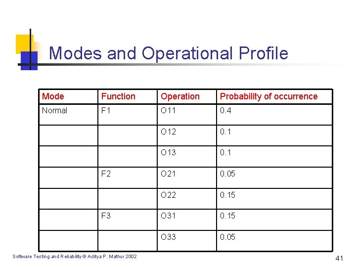
Modes and Operational Profile Mode Function Operation Probability of occurrence Normal F 1 O 11 0. 4 O 12 0. 1 O 13 0. 1 O 21 0. 05 O 22 0. 15 O 31 0. 15 O 33 0. 05 F 2 F 3 Software Testing and Reliability © Aditya P. Mathur 2002 41

Modes and Operational Profile [contd. ] Mode Function Operation Probability of occurrence Administrative AF 1 AO 11 0. 4 AO 12 0. 1 AO 21 0. 5 AF 2 Software Testing and Reliability © Aditya P. Mathur 2002 42

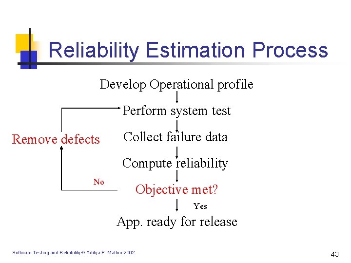
Reliability Estimation Process Develop Operational profile Perform system test Remove defects Collect failure data Compute reliability No Objective met? Yes App. ready for release Software Testing and Reliability © Aditya P. Mathur 2002 43

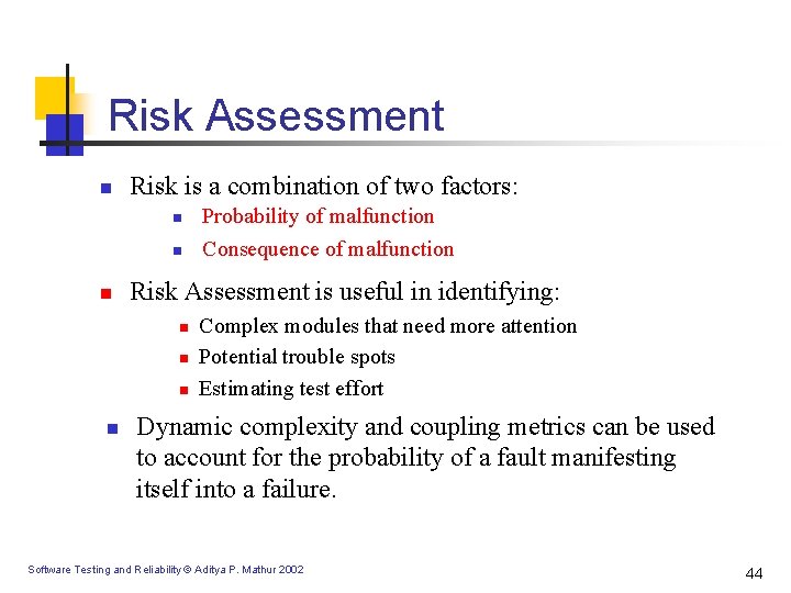
Risk Assessment n Risk is a combination of two factors: n n n Risk Assessment is useful in identifying: n n Probability of malfunction Consequence of malfunction Complex modules that need more attention Potential trouble spots Estimating test effort Dynamic complexity and coupling metrics can be used to account for the probability of a fault manifesting itself into a failure. Software Testing and Reliability © Aditya P. Mathur 2002 44

Question of interest n n Given the architecture of an application, how does one quantify the risk associated with the given architecture? Note that risk analysis, as described here, can be performed prior to the development of any code and soon after the system architecture, in terms of its components and connections, is available. Software Testing and Reliability © Aditya P. Mathur 2002 45

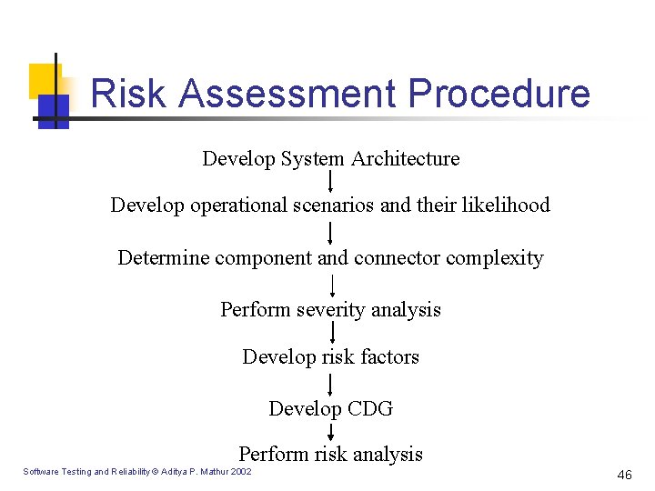
Risk Assessment Procedure Develop System Architecture Develop operational scenarios and their likelihood Determine component and connector complexity Perform severity analysis Develop risk factors Develop CDG Perform risk analysis Software Testing and Reliability © Aditya P. Mathur 2002 46

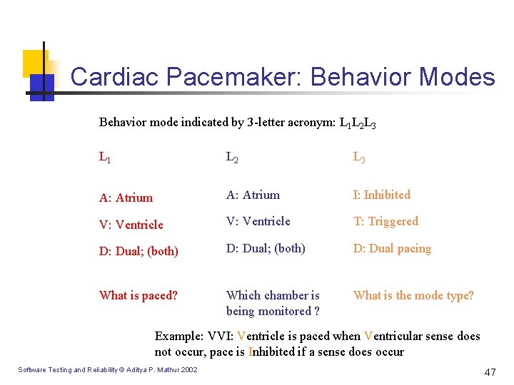
Cardiac Pacemaker: Behavior Modes Behavior mode indicated by 3 -letter acronym: L 1 L 2 L 3 L 1 L 2 L 3 A: Atrium I: Inhibited V: Ventricle T: Triggered D: Dual; (both) D: Dual pacing What is paced? Which chamber is being monitored ? What is the mode type? Example: VVI: Ventricle is paced when Ventricular sense does not occur, pace is Inhibited if a sense does occur Software Testing and Reliability © Aditya P. Mathur 2002 47

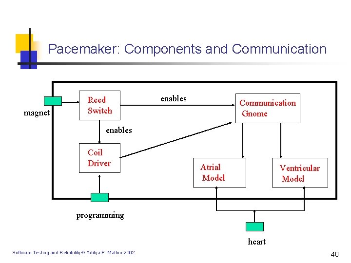
Pacemaker: Components and Communication magnet Reed Switch enables Communication Gnome enables Coil Driver Atrial Model Ventricular Model programming heart Software Testing and Reliability © Aditya P. Mathur 2002 48

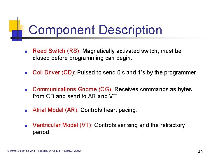
Component Description n n Reed Switch (RS): Magnetically activated switch; must be closed before programming can begin. Coil Driver (CD): Pulsed to send 0’s and 1’s by the programmer. Communications Gnome (CG): Receives commands as bytes from CD and send to AR and VT. Atrial Model (AR): Controls heart pacing. Ventricular Model (VT): Controls sensing and the refractory period. Software Testing and Reliability © Aditya P. Mathur 2002 49

Scenarios n n Programming: Programmer sets the operation mode of the device. AVI: VT monitors the heart. When a heart beat is not sensed the AR paces the heart and a refractory period is in effect. VVI: VT component paces the heart when it does not sense any pulse. AAI: The AR component paces the heart when it does not sense any pulse. n VVT: VT component continuously paces the heart. n AAT: The AR component continuously paces the heart. Software Testing and Reliability © Aditya P. Mathur 2002 50

Static Complexity for OO Designs n n Coupling: Two classes are considered coupled if methods from one class use methods or instance variables from other class. Coupling Between Classes (CBC): Total number of other classes to which a class is coupled. Software Testing and Reliability © Aditya P. Mathur 2002 51

Operational Complexity for Statecharts n n Given a program graph G with e edges and n nodes, the cyclomatic complexity V(G)=e-n+2. Dynamic complexity factor for each component is based on cyclomatic complexity of the statechart specification for each component. For each execution scenario Sk a subset of the statechart specification of the component is executed thereby exercising state entries, state exits, and fired transitions. The cyclomatic complexity of the executed path for each component Ci is called the operational complexity denoted by cpxk (Ci ). Software Testing and Reliability © Aditya P. Mathur 2002 52

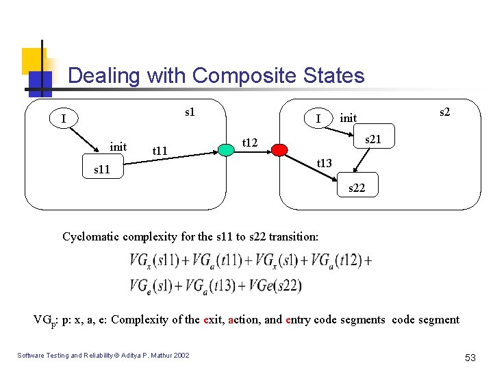
Dealing with Composite States s 1 I init t 11 s 11 I s 2 init s 21 t 12 t 13 s 22 Cyclomatic complexity for the s 11 to s 22 transition: VGp: p: x, a, e: Complexity of the exit, action, and entry code segments code segment Software Testing and Reliability © Aditya P. Mathur 2002 53

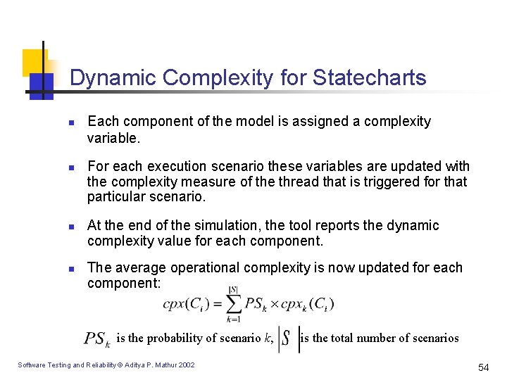
Dynamic Complexity for Statecharts n n Each component of the model is assigned a complexity variable. For each execution scenario these variables are updated with the complexity measure of the thread that is triggered for that particular scenario. At the end of the simulation, the tool reports the dynamic complexity value for each component. The average operational complexity is now updated for each component: is the probability of scenario k, Software Testing and Reliability © Aditya P. Mathur 2002 is the total number of scenarios 54

Component Complexity n n n Sequence diagrams are developed fo each scenario. Each sequence diagram is used to simulate the corresponding scenario. Simulation is used to compute the dynamic complexity of each component. Average operational complexity is then computed as a sum of the scenario component complexity weighted by the scenario probability The component complexities are then normalized against the highest component complexity. Domain experts determine the relative probability of occurrence of each scenario. This is akin to the operational profile of an application. Software Testing and Reliability © Aditya P. Mathur 2002 55

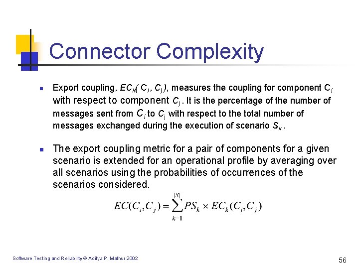
Connector Complexity n n Export coupling, ECk( Ci , Cj ), measures the coupling for component Ci with respect to component Cj. It is the percentage of the number of messages sent from Ci to Cj with respect to the total number of messages exchanged during the execution of scenario Sk. The export coupling metric for a pair of components for a given scenario is extended for an operational profile by averaging over all scenarios using the probabilities of occurrences of the scenarios considered. Software Testing and Reliability © Aditya P. Mathur 2002 56

Connector Complexity n n n Simulation is used to determine the dynamic coupling measure for each connector. Coupling amongst components is represented in the form of a matrix. Coupling values are normalized to the highest coupling. Software Testing and Reliability © Aditya P. Mathur 2002 57

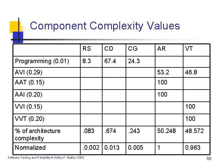
Component Complexity Values AR VT AVI (0. 29) 53. 2 46. 8 AAT (0. 15) 100 AAI (0. 20) 100 Programming (0. 01) RS CD CG 8. 3 67. 4 24. 3 VVI (0. 15) 100 VVT (0. 20) 100 % of architecture complexity . 083 Normalized . 0. 002 0. 013 Software Testing and Reliability © Aditya P. Mathur 2002 . 674 . 243 50. 248 48. 572 0. 005 1 0. 963 58

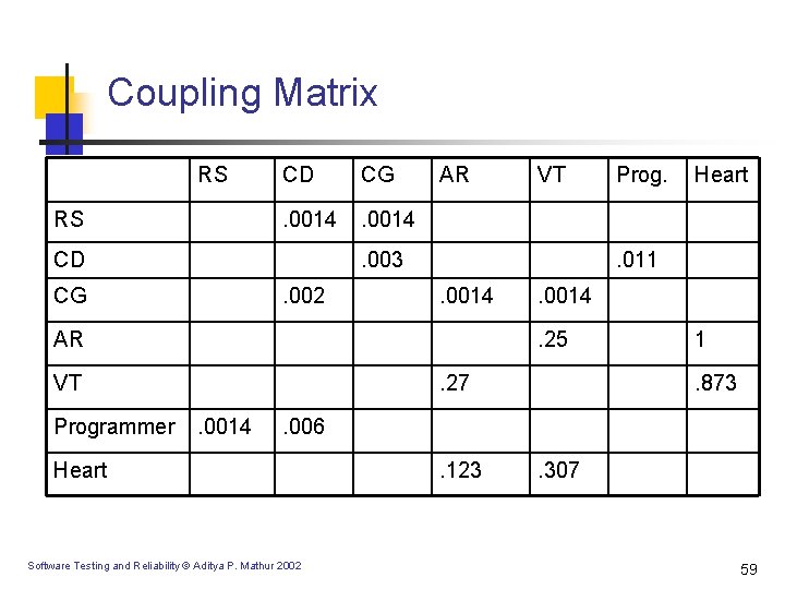
Coupling Matrix RS RS CD CG . 0014 CD AR . 003 CG . 002 . 0014 . 27. 0014 Heart . 0014. 25 VT Prog. . 011 AR Programmer VT 1. 873 . 006 Heart Software Testing and Reliability © Aditya P. Mathur 2002 . 123 . 307 59

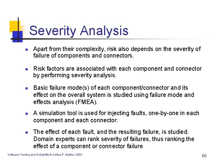
Severity Analysis n n n Apart from their complexity, risk also depends on the severity of failure of components and connectors. Risk factors are associated with each component and connector by performing severity analysis. Basic failure mode(s) of each component/connector and its effect on the overall system is studied using failure mode and effects analysis (FMEA). A simulation tool is used for injecting faults, one-by-one in each component and each connector. The effect of each fault, and the resulting failure, is studied. Domain experts can rank severity of failures, thus ranking the effect of a component or connector failure Software Testing and Reliability © Aditya P. Mathur 2002 60

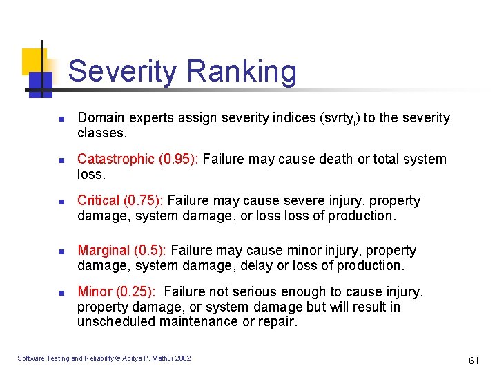
Severity Ranking n n n Domain experts assign severity indices (svrtyi) to the severity classes. Catastrophic (0. 95): Failure may cause death or total system loss. Critical (0. 75): Failure may cause severe injury, property damage, system damage, or loss of production. Marginal (0. 5): Failure may cause minor injury, property damage, system damage, delay or loss of production. Minor (0. 25): Failure not serious enough to cause injury, property damage, or system damage but will result in unscheduled maintenance or repair. Software Testing and Reliability © Aditya P. Mathur 2002 61

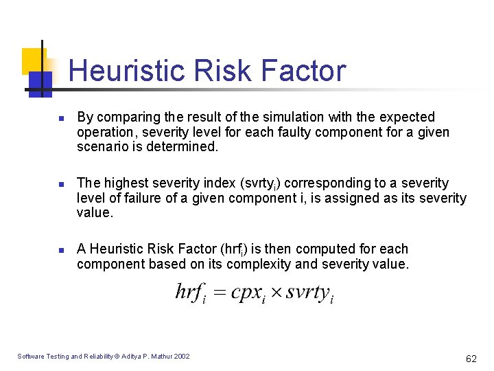
Heuristic Risk Factor n n n By comparing the result of the simulation with the expected operation, severity level for each faulty component for a given scenario is determined. The highest severity index (svrtyi) corresponding to a severity level of failure of a given component i, is assigned as its severity value. A Heuristic Risk Factor (hrfi) is then computed for each component based on its complexity and severity value. Software Testing and Reliability © Aditya P. Mathur 2002 62

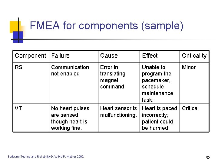
FMEA for components (sample) Component Failure Cause Effect Criticality RS Communication not enabled Error in translating magnet command Unable to program the pacemaker, schedule maintenance task. Minor VT No heart pulses are sensed though heart is working fine. Heart sensor is Heart is paced Critical malfunctioning. incorrectly; patient could be harmed. Software Testing and Reliability © Aditya P. Mathur 2002 63

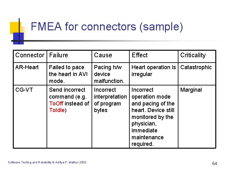
FMEA for connectors (sample) Connector Failure Cause Effect AR-Heart Failed to pace the heart in AVI mode. Pacing h/w device malfunction. Heart operation is Catastrophic irregular CG-VT Send incorrect command (e. g. To. Off instead of To. Idle) Incorrect interpretation of program bytes Incorrect Marginal operation mode and pacing of the heart. Device still monitored by the physician, immediate maintenance required. Software Testing and Reliability © Aditya P. Mathur 2002 Criticality 64

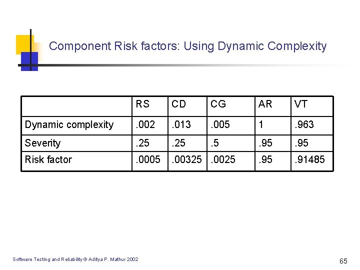
Component Risk factors: Using Dynamic Complexity RS CD CG AR VT Dynamic complexity . 002 . 013 . 005 1 . 963 Severity . 25 . 5 . 95 Risk factor . 0005 . 00325. 0025 . 91485 Software Testing and Reliability © Aditya P. Mathur 2002 65

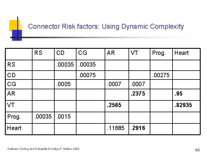
Connector Risk factors: Using Dynamic Complexity RS CD CG RS . 00035 CD . 00075 CG . 0005 AR . 0007 Heart . 0007. 2375 VT Prog. . 00275 AR Prog. VT . 2565 . 95. 82935 . 00035. 0015 Heart Software Testing and Reliability © Aditya P. Mathur 2002 . 11685 . 2916 66

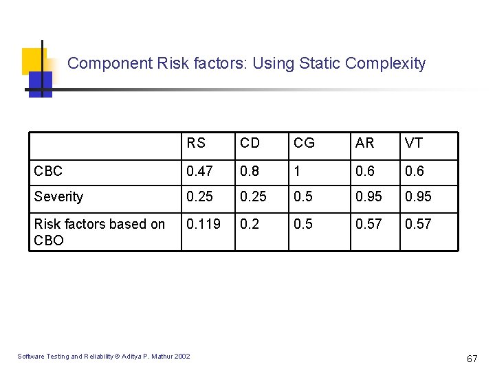
Component Risk factors: Using Static Complexity RS CD CG AR VT CBC 0. 47 0. 8 1 0. 6 Severity 0. 25 0. 95 Risk factors based on CBO 0. 119 0. 2 0. 57 Software Testing and Reliability © Aditya P. Mathur 2002 67

Component Risk factors: Comparison n Dynamic metrics better distinguish AR and VT components as high risk when compared with RS, CD, and CG. Using static metrics, CG is considered at the same risk level as AR and VT. In pacemaker, AR and VT control the heart and hence are the highest risk components which is confirmed when one computes the risk factors using dynamic metrics. Software Testing and Reliability © Aditya P. Mathur 2002 68

Component Dependency Graphs (CDGs) n n A CDG is described by sets N and E where N is a set of of nodes and E is a set of edges. s and t are designated as the start and termination nodes and belong to N. Each node n in N: <Ci, RCi, ECi>, where Ci is the component corresponding to n, RCi is the reliability of Ci , and ECi is the average execution time of Ci. Each edge e in E : <Tij , RTij , PTi j>, where Tij is the transition from node Ci to Cj, RTij is the reliability of this transition, and PTi j is the transition probability. In the methodology described here, risk factors replace the reliabilities of components and transitions. Software Testing and Reliability © Aditya P. Mathur 2002 69

Generation of CDGs n n Estimate the execution probability of each scenario. For each scenario estimate the execution time of each component and then, using the probability of each scenario, compute the average execution time of each component. n Estimate the transition probability of each transition. n Estimate the complexity factor of each component. n Estimate the complexity factor of each connector. . Software Testing and Reliability © Aditya P. Mathur 2002 70

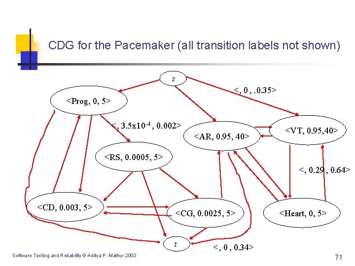
CDG for the Pacemaker (all transition labels not shown) s <, 0 , . 0. 35> <Prog, 0, 5> <, 3. 5 x 10 -4 , 0. 002> <AR, 0. 95, 40> <VT, 0. 95, 40> <RS, 0. 0005, 5> <, 0. 29 , 0. 64> <CD, 0. 003, 5> <CG, 0. 0025, 5> t Software Testing and Reliability © Aditya P. Mathur 2002 <Heart, 0, 5> <, 0 , 0. 34> 71

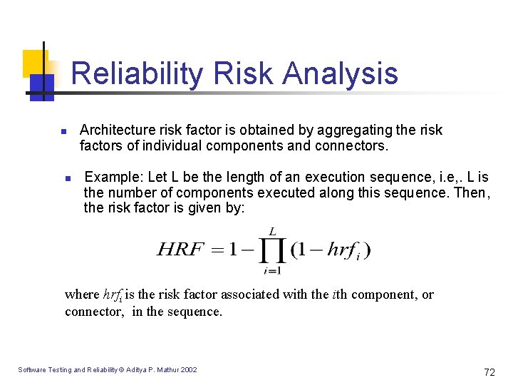
Reliability Risk Analysis n n Architecture risk factor is obtained by aggregating the risk factors of individual components and connectors. Example: Let L be the length of an execution sequence, i. e, . L is the number of components executed along this sequence. Then, the risk factor is given by: where hrfi is the risk factor associated with the ith component, or connector, in the sequence. Software Testing and Reliability © Aditya P. Mathur 2002 72

Risk Analysis Algorithm-OR paths n n Traverse the CDG starting at node s and stop until either t is reached or the average application execution time is consumed. Breadth expansions correspond to “OR” paths. The risk factors associated with all nodes along the breadth expansion are summed up weighted by the transition probabilities. s e 1: <(s, n 1), 0, 0. 3> e 1 e 2: <(s, n 2), 0, 0. 7> n 1: <(C 1, 0. 5, 5 > n 2: <(C 2, 0. 6, 12 > n n 1 e 2 n 2 HRF=1 -[(1 -0. 5)0. 3+(1 -0. 6)0. 7]. Software Testing and Reliability © Aditya P. Mathur 2002 73

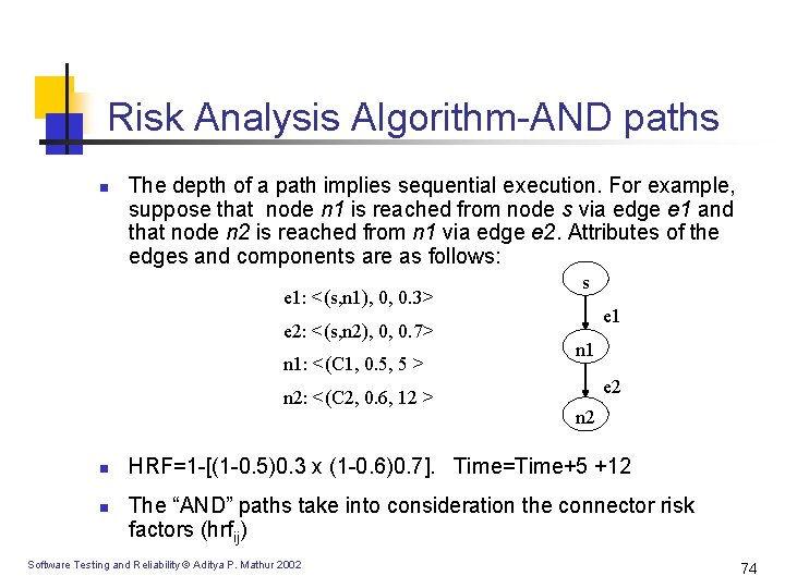
Risk Analysis Algorithm-AND paths n The depth of a path implies sequential execution. For example, suppose that node n 1 is reached from node s via edge e 1 and that node n 2 is reached from n 1 via edge e 2. Attributes of the edges and components are as follows: e 1: <(s, n 1), 0, 0. 3> e 2: <(s, n 2), 0, 0. 7> n 1: <(C 1, 0. 5, 5 > n 2: <(C 2, 0. 6, 12 > n n s e 1 n 1 e 2 n 2 HRF=1 -[(1 -0. 5)0. 3 x (1 -0. 6)0. 7]. Time=Time+5 +12 The “AND” paths take into consideration the connector risk factors (hrfij) Software Testing and Reliability © Aditya P. Mathur 2002 74

Pacemaker Risk n n Given the architecture and the risk factors associated with components and connector, the risk factor associated with the pacemaker is computed to be approx. 0. 9. This value of risk is considered high. It implies that the pacemaker architecture is critical and failures are likely to be catastrophic. Risk analysis tells us that the VT and AR components are the highest risk components Risk analysis also tells us that the connectors between VT, AR and heart components are the highest risk components Software Testing and Reliability © Aditya P. Mathur 2002 75

Advantages of Risk Analysis n n n The CDG is useful for the risk analysis of hierarchical systems. Risks for subsystems can be computed. These could then be aggregated to compute then risk of the entire system. The CDG is useful for performing sensitivity analysis. One could study the impact of changing the risk factor of a component on the risk associated with the entire system. As the analysis is being done, most likely, prior to coding, one might consider revising the architecture or use the same architecture but allocate resources for coding and testing based on individual risk factors. Software Testing and Reliability © Aditya P. Mathur 2002 76

Summary n n Reliability, modeling uncertainty, failure intensity, operational profile, reliability growth models, parameter estimation. Risk assessment, architecture, severity analysis, risk factors, CDGs. Software Testing and Reliability © Aditya P. Mathur 2002 77