Software Reliability Growth Models Introduction Software reliability growth
Software Reliability Growth Models
Introduction “Software reliability growth models can be used as an indication of the number of failures that may be encountered after the software has shipped and thus as an indication of whether the software is ready to ship; These models use system test data to predict the number of defects remaining in the software” 2
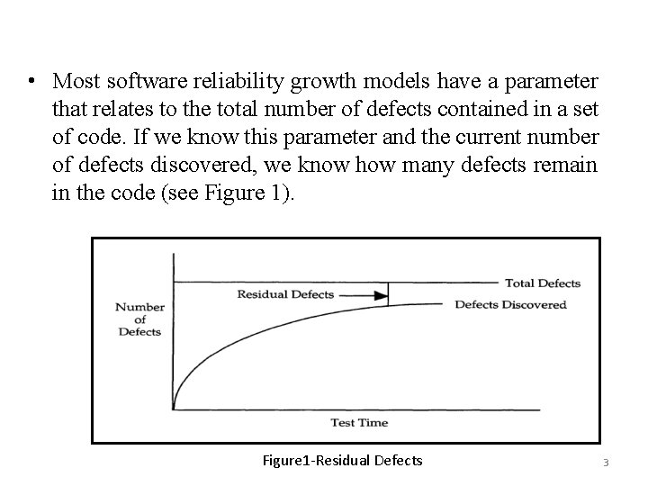
• Most software reliability growth models have a parameter that relates to the total number of defects contained in a set of code. If we know this parameter and the current number of defects discovered, we know how many defects remain in the code (see Figure 1). Figure 1 -Residual Defects 3
• Knowing the number of residual defects helps us decide whether or not the code is ready to ship and how much more testing is required if we decide the code is not ready to ship. It gives us an estimate of the number of failures that our customers will encounter when operating the software. “Software reliability growth models are a statistical interpolation of defect detection data by mathematical functions. The functions are used to predict future failure rates or the number of residual defects in the code. ” [Alan Wood , Tandem Software Reliability Growth Models] 4
Software Reliability Growth Model Data 1. Test Time Data-For a software reliability growth model developed during QA test, the appropriate measure of time must relate to the testing effort. There are three possible candidates for measuring test time: - calendar time - number of tests run - execution (CPU) time. 5
2. Defect Data. Major: Can tolerate the situation, but not for long. Solution needed. Critical: Intolerable situation. Solution urgently needed. 3. Grouped Datathe amount of failures and test time that occurred during a week. 6
Software Reliability Growth Model Types Software reliability growth models have been grouped into two classes of models concave and S-shaped (figure 2) The most important thing about both models is that they have the same asymptotic behavior, i. e. , the defect detection rate decreases as the number of defects detected (and repaired) increases, and the total number of defects detected asymptotically approaches a finite value. 7
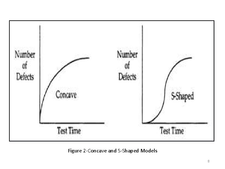
Figure 2 -Concave and S-Shaped Models 8
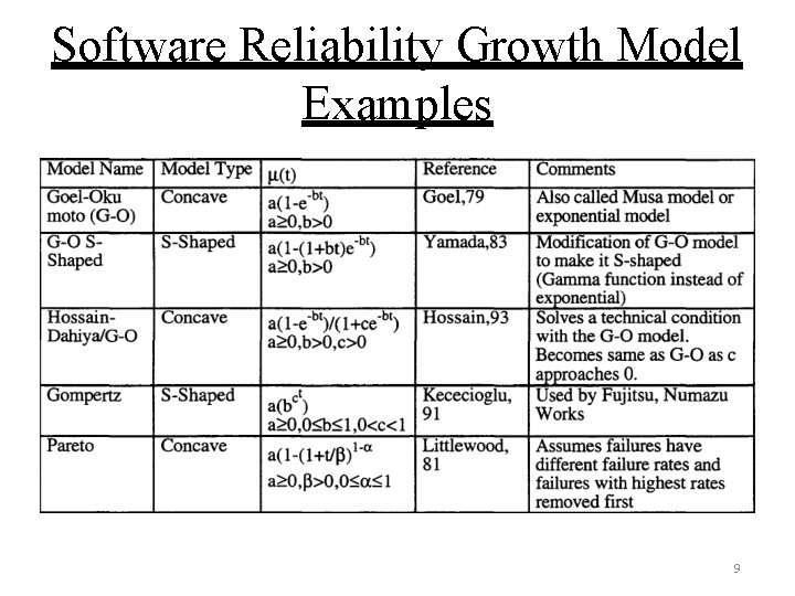
Software Reliability Growth Model Examples 9
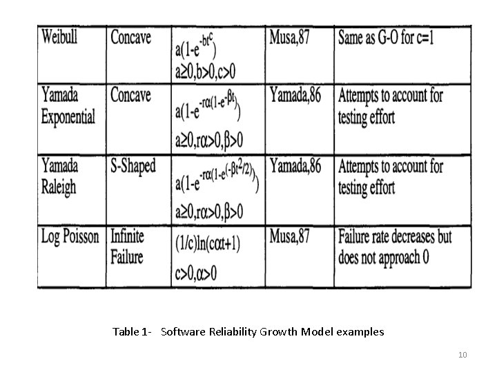
Table 1 - Software Reliability Growth Model examples 10
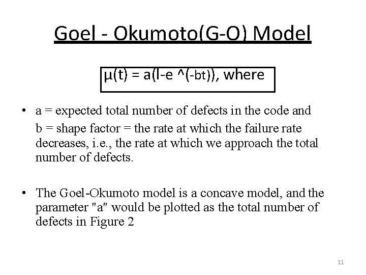
Goel - Okumoto(G-O) Model μ(t) = a(l-e ^(-bt)), where • a = expected total number of defects in the code and b = shape factor = the rate at which the failure rate decreases, i. e. , the rate at which we approach the total number of defects. • The Goel-Okumoto model is a concave model, and the parameter "a" would be plotted as the total number of defects in Figure 2 11
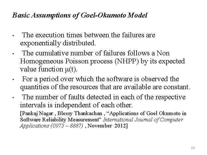
Basic Assumptions of Goel-Okumoto Model • • The execution times between the failures are exponentially distributed. The cumulative number of failures follows a Non Homogeneous Poisson process (NHPP) by its expected value function μ(t). For a period over which the software is observed the quantities of the resources that are available are constant. The number of faults detected in each of the respective intervals is independent of each other. [Pankaj Nagar , Blessy Thankachan , “Applications of Goel Okumoto in Software Reliability Measurement” International Journal of Computer Applications (0975 – 8887) , November 2012] 12

Thank You 13
- Slides: 13