Software Metrics and Design Principles What is Design

Software Metrics and Design Principles

What is Design? • Design is the process of creating a plan or blueprint to follow during actual construction • Design is a problem-solving activity that is iterative in nature • In traditional software engineering the outcome of design is the design document or technical specification (if emphasis on notation)

“Wicked Problem” • Software design is a “Wicked Problem” – Design phase can’t be solved in isolation • Designer will likely need to interact with users for requirements, programmers for implementation – No stopping rule • How do we know when the solution is reached? – Solutions are not true or false • Large number of tradeoffs to consider, many acceptable solutions – Wicked problems are a symptom of another problem • Resolving one problem may result in a new problem elsewhere; software is not continuous

Systems-Oriented Approach • The central question: how to decompose a system into parts such that each part has lower complexity than the system as a whole, while the parts together solve the user’s problem? • In addition, the interactions between the components should not be too complicated • Vast number of design methods exist

Design Considerations • “Module” used often – usually refers to a method or class • In the decomposition we are interested in properties that make the system flexible, maintainable, reusable – – – Information Hiding System Structure Complexity Abstraction Modularity

Abstraction • Abstraction – Concentrate on the essential features and ignore, abstract from, details that are not relevant at the level we are currently working on – E. g. Sorting Module • Consider inputs, outputs, ignore details of the algorithms until later – Two general types of abstraction • Procedural Abstraction • Data Abstraction

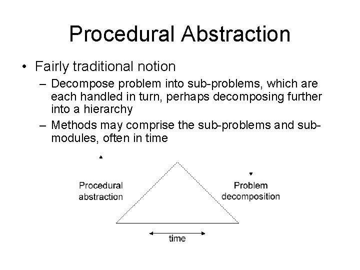
Procedural Abstraction • Fairly traditional notion – Decompose problem into sub-problems, which are each handled in turn, perhaps decomposing further into a hierarchy – Methods may comprise the sub-problems and submodules, often in time

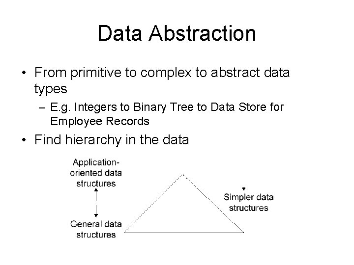
Data Abstraction • From primitive to complex to abstract data types – E. g. Integers to Binary Tree to Data Store for Employee Records • Find hierarchy in the data

Modularity • During design the system is decomposed into modules and the relationships among modules are indicated • Two structural design criteria as to the “goodness” of a module – Cohesion : Glue for intra-module components – Coupling : Strength of inter-module connections

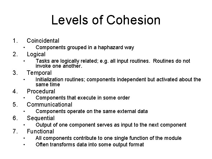
Levels of Cohesion 1. Coincidental • 2. Components grouped in a haphazard way Logical • 3. Tasks are logically related; e. g. all input routines. Routines do not invoke one another. Temporal • 4. Initialization routines; components independent but activated about the same time Procedural • 5. Components that execute in some order Communicational • 6. Components operate on the same external data Sequential • 7. Output of one component serves as input to the next component Functional • • All components contribute to one single function of the module Often transforms data into some output format

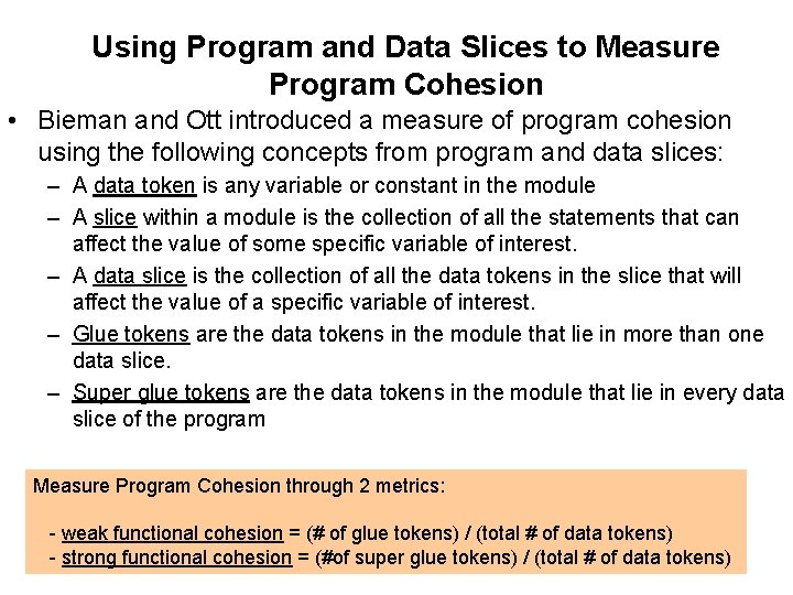
Using Program and Data Slices to Measure Program Cohesion • Bieman and Ott introduced a measure of program cohesion using the following concepts from program and data slices: – A data token is any variable or constant in the module – A slice within a module is the collection of all the statements that can affect the value of some specific variable of interest. – A data slice is the collection of all the data tokens in the slice that will affect the value of a specific variable of interest. – Glue tokens are the data tokens in the module that lie in more than one data slice. – Super glue tokens are the data tokens in the module that lie in every data slice of the program Measure Program Cohesion through 2 metrics: - weak functional cohesion = (# of glue tokens) / (total # of data tokens) - strong functional cohesion = (#of super glue tokens) / (total # of data tokens)

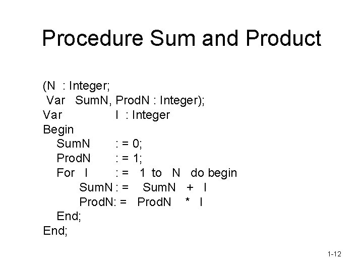
Procedure Sum and Product (N : Integer; Var Sum. N, Prod. N : Integer); Var I : Integer Begin Sum. N : = 0; Prod. N : = 1; For I : = 1 to N do begin Sum. N : = Sum. N + I Prod. N: = Prod. N * I End; 1 -12

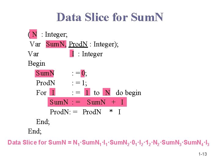
Data Slice for Sum. N ( N : Integer; Var Sum. N, Prod. N : Integer); Var I : Integer Begin Sum. N : = 0; Prod. N : = 1; For I : = 1 to N do begin Sum. N : = Sum. N + I Prod. N: = Prod. N * I End; Data Slice for Sum. N = N 1·Sum. N 1·I 1·Sum. N 2· 01·I 2· 12·N 2·Sum. N 3·Sum. N 4·I 3 1 -13

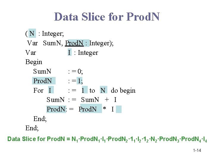
Data Slice for Prod. N ( N : Integer; Var Sum. N, Prod. N : Integer); Var I : Integer Begin Sum. N : = 0; Prod. N : = 1; For I : = 1 to N do begin Sum. N : = Sum. N + I Prod. N: = Prod. N * I End; Data Slice for Prod. N = N 1·Prod. N 1·I 1·Prod. N 2· 11·I 2· 12·N 2·Prod. N 3·Prod. N 4·I 4 1 -14

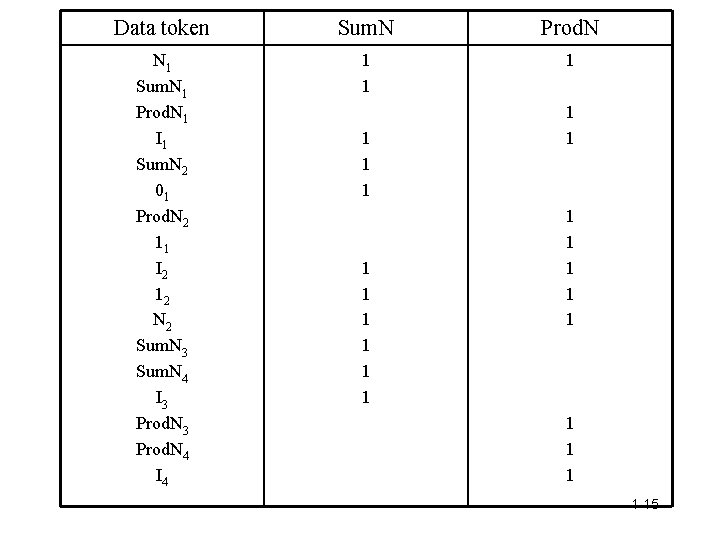
Data token Sum. N Prod. N N 1 Sum. N 1 Prod. N 1 I 1 Sum. N 2 01 Prod. N 2 11 I 2 12 N 2 Sum. N 3 Sum. N 4 I 3 Prod. N 4 I 4 1 1 1 1 1 1 -15

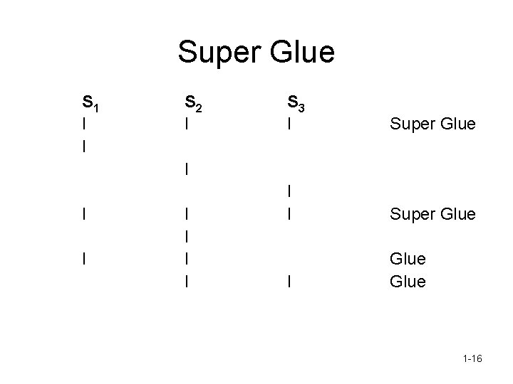
Super Glue S 1 I I S 2 I S 3 I Super Glue I I I I 1 -16

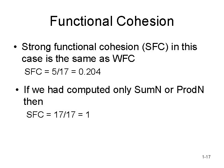
Functional Cohesion • Strong functional cohesion (SFC) in this case is the same as WFC SFC = 5/17 = 0. 204 • If we had computed only Sum. N or Prod. N then SFC = 17/17 = 1 1 -17

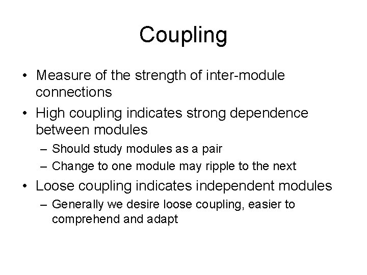
Coupling • Measure of the strength of inter-module connections • High coupling indicates strong dependence between modules – Should study modules as a pair – Change to one module may ripple to the next • Loose coupling indicates independent modules – Generally we desire loose coupling, easier to comprehend adapt

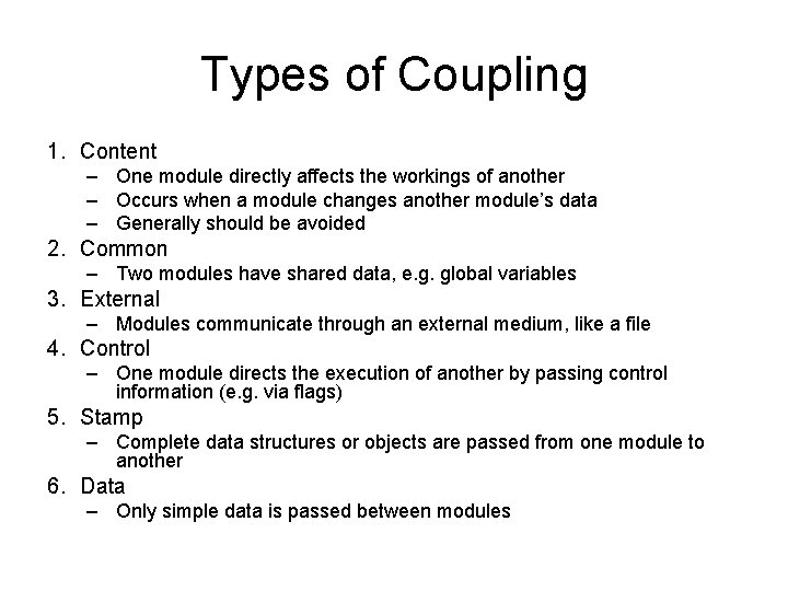
Types of Coupling 1. Content – One module directly affects the workings of another – Occurs when a module changes another module’s data – Generally should be avoided 2. Common – Two modules have shared data, e. g. global variables 3. External – Modules communicate through an external medium, like a file 4. Control – One module directs the execution of another by passing control information (e. g. via flags) 5. Stamp – Complete data structures or objects are passed from one module to another 6. Data – Only simple data is passed between modules

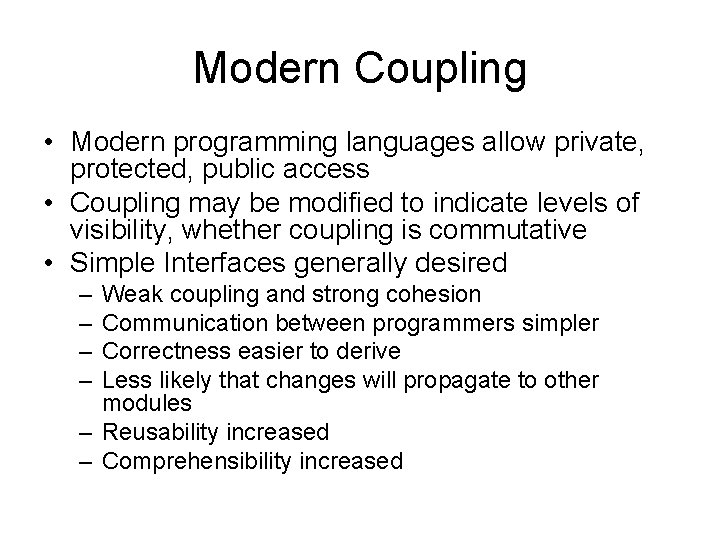
Modern Coupling • Modern programming languages allow private, protected, public access • Coupling may be modified to indicate levels of visibility, whether coupling is commutative • Simple Interfaces generally desired – – Weak coupling and strong cohesion Communication between programmers simpler Correctness easier to derive Less likely that changes will propagate to other modules – Reusability increased – Comprehensibility increased

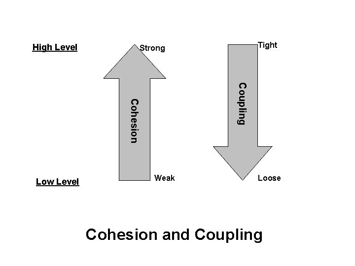
High Level Coupling Cohesion Low Level Tight Strong Weak Loose Cohesion and Coupling

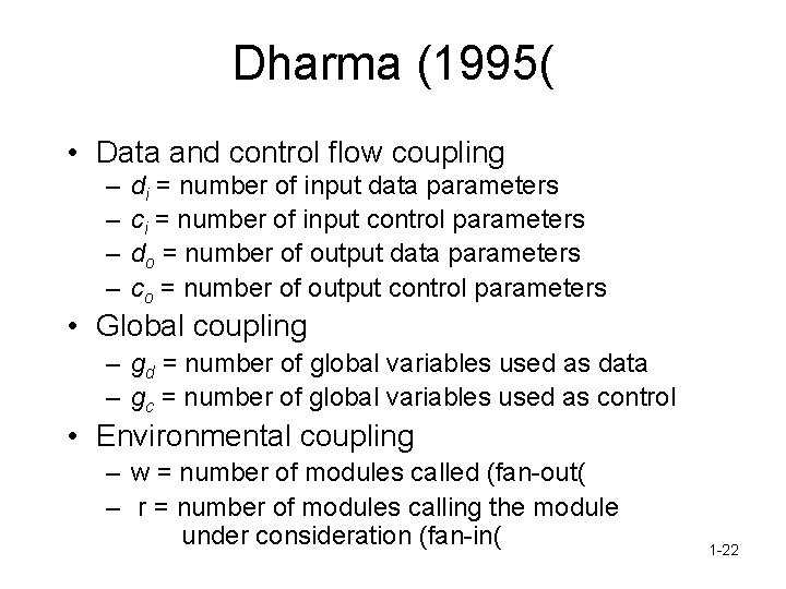
Dharma (1995( • Data and control flow coupling – – di = number of input data parameters ci = number of input control parameters do = number of output data parameters co = number of output control parameters • Global coupling – gd = number of global variables used as data – gc = number of global variables used as control • Environmental coupling – w = number of modules called (fan-out( – r = number of modules calling the module under consideration (fan-in( 1 -22

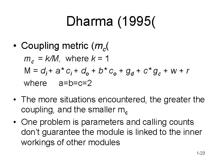
Dharma (1995( • Coupling metric (mc( mc = k/M, where k = 1 M = di + a* ci + do + b* co + gd + c* gc + w + r where a=b=c=2 • The more situations encountered, the greater the coupling, and the smaller mc • One problem is parameters and calling counts don’t guarantee the module is linked to the inner workings of other modules 1 -23

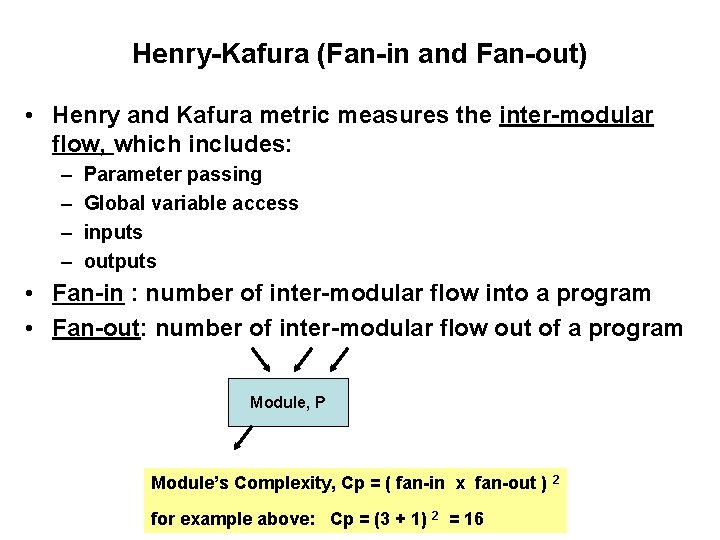
Henry-Kafura (Fan-in and Fan-out) • Henry and Kafura metric measures the inter-modular flow, which includes: – – Parameter passing Global variable access inputs outputs • Fan-in : number of inter-modular flow into a program • Fan-out: number of inter-modular flow out of a program Module, P Module’s Complexity, Cp = ( fan-in x fan-out ) for example above: Cp = (3 + 1) 2 = 16 2

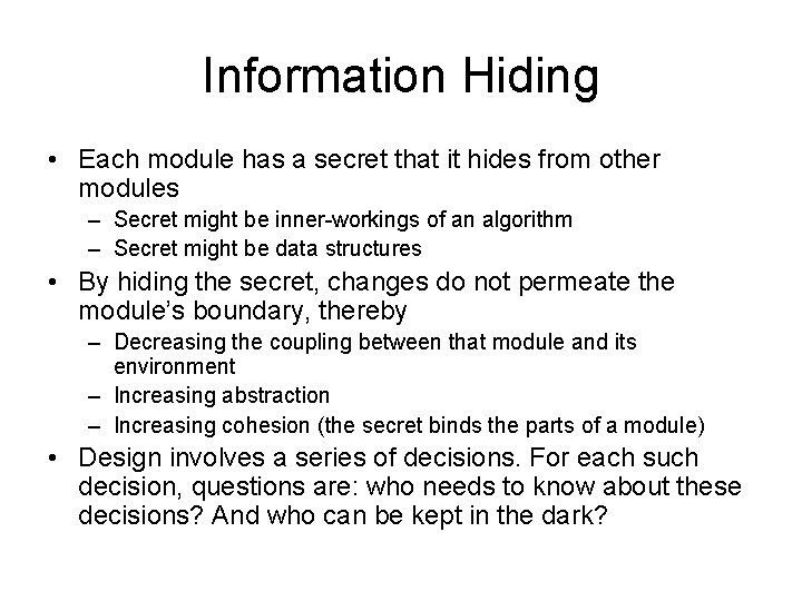
Information Hiding • Each module has a secret that it hides from other modules – Secret might be inner-workings of an algorithm – Secret might be data structures • By hiding the secret, changes do not permeate the module’s boundary, thereby – Decreasing the coupling between that module and its environment – Increasing abstraction – Increasing cohesion (the secret binds the parts of a module) • Design involves a series of decisions. For each such decision, questions are: who needs to know about these decisions? And who can be kept in the dark?

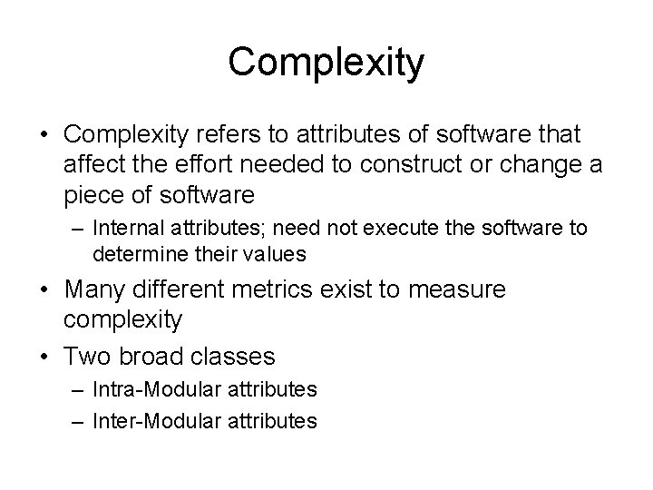
Complexity • Complexity refers to attributes of software that affect the effort needed to construct or change a piece of software – Internal attributes; need not execute the software to determine their values • Many different metrics exist to measure complexity • Two broad classes – Intra-Modular attributes – Inter-Modular attributes

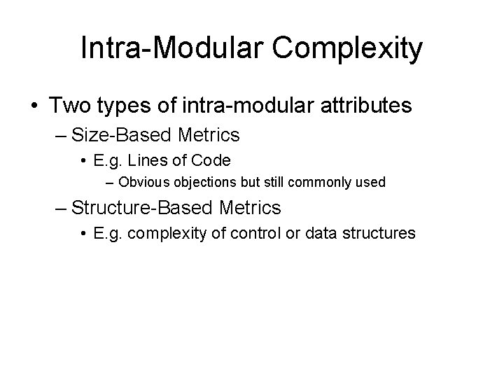
Intra-Modular Complexity • Two types of intra-modular attributes – Size-Based Metrics • E. g. Lines of Code – Obvious objections but still commonly used – Structure-Based Metrics • E. g. complexity of control or data structures

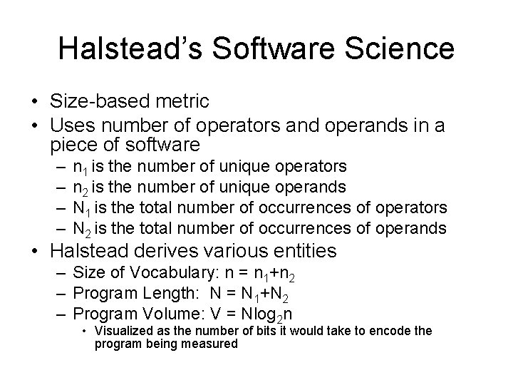
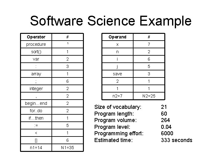
Halstead’s Software Science • Size-based metric • Uses number of operators and operands in a piece of software – – n 1 is the number of unique operators n 2 is the number of unique operands N 1 is the total number of occurrences of operators N 2 is the total number of occurrences of operands • Halstead derives various entities – Size of Vocabulary: n = n 1+n 2 – Program Length: N = N 1+N 2 – Program Volume: V = Nlog 2 n • Visualized as the number of bits it would take to encode the program being measured

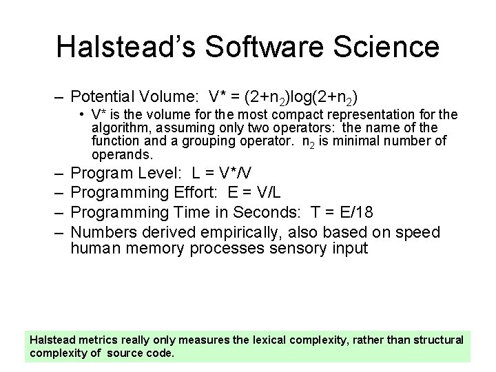
Halstead’s Software Science – Potential Volume: V* = (2+n 2)log(2+n 2) • V* is the volume for the most compact representation for the algorithm, assuming only two operators: the name of the function and a grouping operator. n 2 is minimal number of operands. – – Program Level: L = V*/V Programming Effort: E = V/L Programming Time in Seconds: T = E/18 Numbers derived empirically, also based on speed human memory processes sensory input Halstead metrics really only measures the lexical complexity, rather than structural complexity of source code.

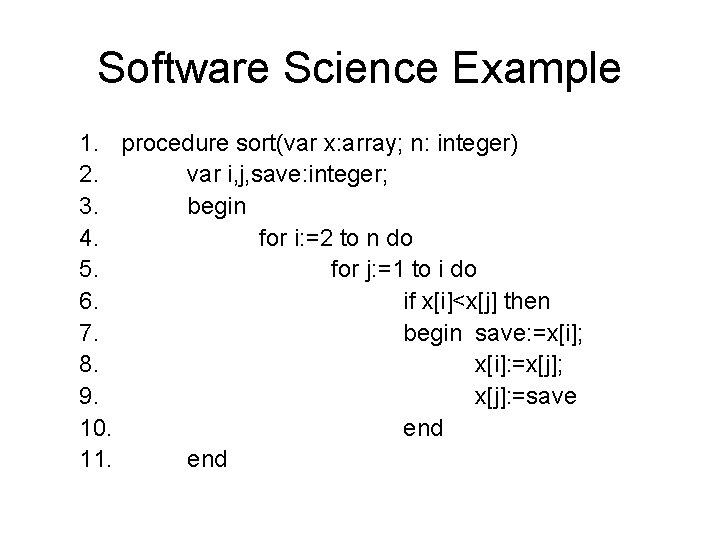
Software Science Example 1. procedure sort(var x: array; n: integer) 2. var i, j, save: integer; 3. begin 4. for i: =2 to n do 5. for j: =1 to i do 6. if x[i]<x[j] then 7. begin save: =x[i]; 8. x[i]: =x[j]; 9. x[j]: =save 10. end 11. end

Software Science Example Operator # Operand # procedure 1 x 7 sort() 1 n 2 var 2 i 6 : 3 j 5 array 1 save 3 ; 6 2 1 integer 2 1 1 , 2 n 2=7 N 2=25 begin…end 2 for. . do 2 if…then 1 : = 5 < 1 [] 6 n 1=14 N 1=35 Size of vocabulary: Program length: Program volume: Program level: Programming effort: Estimated time: 21 60 264 0. 04 6000 333 seconds

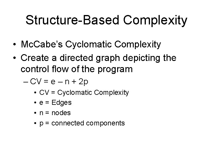
Structure-Based Complexity • Mc. Cabe’s Cyclomatic Complexity • Create a directed graph depicting the control flow of the program – CV = e – n + 2 p • • CV = Cyclomatic Complexity e = Edges n = nodes p = connected components

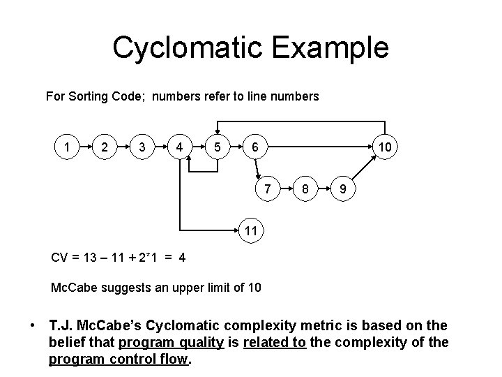
Cyclomatic Example For Sorting Code; numbers refer to line numbers 1 2 3 4 5 6 10 7 8 9 11 CV = 13 – 11 + 2*1 = 4 Mc. Cabe suggests an upper limit of 10 • T. J. Mc. Cabe’s Cyclomatic complexity metric is based on the belief that program quality is related to the complexity of the program control flow.

Shortcomings of Complexity Metrics • Not context-sensitive – Any program with five if-statements has the same cyclomatic complexity – Measure only a few facts; e. g. Halstead’s method doesn’t consider control flow complexity • Others? • Minix: – Of the 277 modules, 34 have a CV > 10 – Highest has 58; handles ASCII escape sequences. A review of the module was deemed “justifiably complex”; attempts to reduce complexity by splitting into modules would increase difficulty to understand artificially reduce the CV

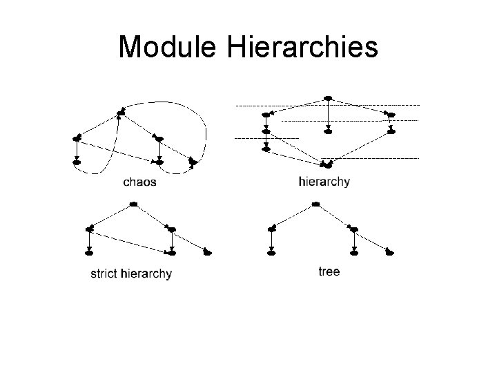
System Structure – Inter-Module Complexity • The design may consist of modules and their relationships • Can denote this in a graph; nodes are modules and edges are relationships between modules • Types of inter-module relationships: – – Module A contains Module B Module A follows Module B Module A delivers data to Module B Module A uses Module B • We are mostly interested in the last one, which manifests itself via a call graph – Possible shapes: • • Chaotic Directed Acyclic Graph (Hierarchy) Layered Graph (Strict Hierarchy) Tree

Module Hierarchies

Graph Metrics • Metrics use: – Size of the graph – Depth – Width (maximum number of nodes at some level) • A tree-like call graph is considered the best design – Some metrics measure the deviation from a tree; the tree impurity of the graph – Compute number of edges that must be removed from the graph’s minimum spanning tree • Other metrics – Complexity(M) = fanin(M)*fanout(M) – Fanin/Fanout = local and global data flows

Software Metrics Etiquette • Use common sense and organizational sensitivity when interpreting metrics data. • Provide regular feedback to the individuals and teams who have worked to collect measures and metrics. • Don’t use metrics to appraise individuals • Work with practitioners and teams to set clear goals and metrics that will be used to achieve them. • Never use metrics to threaten individuals or teams. • Metrics data that indicate a problem area should not be considered “negative”. These data are merely an indicator for process improvement. • Don’t obsess on a single metric to the exclusion of other important metrics. 1 -38