SOFTWARE MEASUREMENT AND METRICS 1 Software Measurement is

SOFTWARE MEASUREMENT AND METRICS 1

Software Measurement is the process by which numbers or symbols are assigned to attributes of entities in the real world in such a way as to describe them according to clearly defined unambiguous rules. Metrics and measurements are necessary aspects of managing a software development project. For effective monitoring, management needs to get information about the project: § § how far it has progressed how much development has taken place how far behind schedule it is, and the quality of the development so far Based on this information, decisions, can be made about the project. 2

Types of Measurement can be categorized in two ways : - 1. Direct Measures 2. Indirect Measures 3

Software Metrics: What and Why ? Software metric is defined as a quantitative measure of an attribute a software system possesses with respect to Cost, Quality, Size and Schedule. Example. Measure - No. of Errors Metrics - No. of Errors found person These are numerical data related to software development. Metrics strongly support software project management activities. 4

1. How to measure the size of a software? 2. How much will it cost to develop a software? 3. How many bugs can we expect? 4. When can we stop testing? 5. When can we release the software?

6. What is the complexity of a module? 7. What is the module strength and coupling? 8. What is the reliability at the time of release? 9. Which test technique is more effective? 10. Are we testing hard or are we testing smart? 11. Do we have a strong program or a week test suite? 6

❖ Pressman explained as “A measure provides a quantitative indication of the extent, amount, dimension, capacity, or size of some attribute of the product or process”. ❖ Measurement is the act of determine a measure ❖ The metric is a quantitative measure of the degree to which a system, component, or process possesses a given attribute. ❖ Fenton defined measurement as “ it is the process by which numbers or symbols are assigned to attributes of entities in the real world in such a way as to describe them according to clearly defined rules”. 7

Areas of Applications The most established area of software metrics is cost and size estimation techniques. The prediction of quality levels for software, often in terms of reliability, is another area where software metrics have an important role to play. The use of software metrics to provide quantitative checks on software design is also a well established area. 8

Categories of Metrics i. Product metrics: describe the characteristics of the product such as size, complexity, design features, performance, efficiency, reliability, portability, etc. ii. Process metrics: describe the effectiveness and quality of the processes that produce the software product. Examples are: • effort required in the process • time to produce the product • effectiveness of defect removal during development • number of defects found during testing 9

iii. Project metrics: describe the project characteristics and execution. Examples are : • number of software developers • cost and schedule • productivity 10

Control flow graph A control flow graph (CFG) describes: §the sequence in which different instructions of a program get executed. §the way control flows through the program. Control flow depicts a program as a graph which consists of Nodes and Edges.

In the graph, Nodes represent processing tasks while edges represent control flow between the nodes.

Flow graph notation for a program: 50

How to draw Control flow graph? §Number all the statements of a program. §Numbered statements: - represent nodes of the control flow graph. §An edge from one node to another node exists: - if execution of the statement representing the first node can result in transfer of control to the other node.

Example int f 1(int x, int y){ 1. while (x != y){ 2. if (x>y) then 3. x=x-y; 4. else y=y-x; 5. } 6. return x; }

Example Control Flow Graph 1 2 3 4 5 6 Cyclomatic complexity = 7 – 6 + 2 = 3.

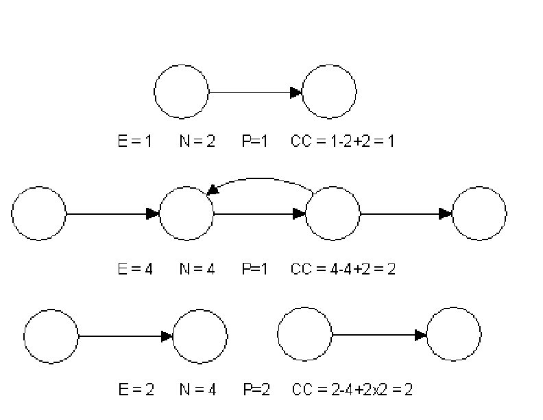
CYCLOMATIC COMPLEXITY This metric was developed by Thomas J. Mc. Cabe in 1976 and it is based on a control flow representation of the program. Mc. Cabe's cyclomatic complexity is a software quality metric that quantifies the complexity of a software program. Complexity is inferred by measuring the number of linearly independent paths through the program. The higher the number the more complex the code. Independent path is defined as a path that has atleast one edge which has not been traversed before in any other paths. Cyclomatic complexity can be calculated with respect to functions, modules, methods or classes within a program. 50

Different ways to compute CC There are three methods: Method 1: Cyclomatic complexity is derived from the control flow graph of a program as follows: Cyclomatic complexity(CC), V(G) = E - N + 2 P Where: E = number of edges (transfers of control) N = number of nodes (sequential group of statements containing only one transfer of control) P = number of disconnected parts of the flow graph (e. g. a calling program and a subroutine) or number of strongly connected components 50

Different ways to compute CC Method 2: An alternative way of computing the Cyclomatic complexity of a program from an inspection of its control flow graph is as follows: V(G) = Total number of bounded areas + 1 • Any region enclosed by nodes and edges can be called as a bounded area. Method 3: Cyclomatic complexity can also be computed by computing the number of decision statements. V (G) = Π + 1 Where Π = number of decision statement of a program. 50

Flow graph for program will be 50

Flow graph notation Computing mathematically, V(G) = 9 - 7 + 2 = 4 V(G) = 3 + 1 = 4 (Condition nodes are 1, 2 and 3 nodes) Basis Set - A set of possible execution path of a program or There will be four independent paths for the flow graph. Path 1: 1, 7 Path 2: 1, 2, 6, 1, 7 Path 3: 1, 2, 3, 4, 5, 2, 6, 1, 7 Path 4: 1, 2, 3, 5, 2, 6, 1, 7 50

Properties of Cyclomatic complexity: Following are the properties of Cyclomatic complexity: 1. V (G) >=1 2. V (G) is the maximum number of independent paths in the graph 3. Inserting and deleting functional statements to G does not affect V(G) 4. G will have only one path if and only if V (G) = 1 5. Inserting a new row in G increases V(G) by unity. 50

Example

SOLUTION It can be calculated by any of the three methods 1. V(G) = E – N + 2 P = 13 – 10 + 2 = 5 2. V(G) = Π + 1 = 4 + 1 = 5 3. V(G) = no. of regions + 1; = 4 + 1 = 5 50

HALSTEAD’s SOFTWARE SCIENCE METRICS It is an analytical technique to measure size, development effort and development cost of software products. Halstead used a few primitive program parameters to develop the expressions for overall program length, potential minimum value, actual volume, effort and development time. 26

Token Count The size of the vocabulary of a program, which consists of the number of unique tokens used to build a program is defined as: = 1+ 2 where : vocabulary of a program 1 : number of unique operators 2 : number of unique operands 27

The length of the program in the terms of the total number of tokens used is N = N 1+N 2 where N : program length N 1 : total occurrences of operators N 2 : total occurrences of operands 28

Program Volume V = N * log 2 The unit of measurement of volume is the common unit for size “bits”. It is the actual size of a program if a uniform binary encoding for the vocabulary is used. Program Length Equation N` = 1 log 2 1 + 2 log 2 2 ` on N means it is calculated rather than counted 29

Potential Volume V* = ( 1* + 2*) log 2 ( 1* + 2*) where 1* = 2 2* represents the no. of conceptually unique input and output parameters. Program Level L = V* / V The value of L ranges between zero and one, with L=1 representing a program written at the highest possible level (i. e. , with minimum size). 30

Program Difficulty D=1/L As the volume of an implementation of a program increases, the program level decreases and the difficulty increases. Thus, programming practices such as redundant usage of operands, or the failure to use higher-level control constructs will tend to increase the volume as well as the difficulty. Effort Equation E=V/L=D*V The unit of measurement of E is elementary mental discriminations. 31

Time equation T’ = E/S John Stroud defined a moment as the time required by the human brain to perform the most elementary discrimination. The Stroud number S is 18. . 32

Advantages of Halstead Metrics Ø Simple to calculate Ø Do not require in-depth analysis of programming structure. Ø Measure overall quality of programs. Ø Predicts maintenance efforts. Ø Useful in scheduling the projects. 33

Counting rules for C language 1. Comments are not considered. 2. All the variables and constants are considered operands. 3. Global variables used in different modules of the same program are counted as multiple occurrences of the same variable. 34

4. Local variables with the same name in different functions are counted as unique operands. 5. Functions calls are considered as operators. 6. All looping statements e. g. , do {…} while ( ), while ( ) {…}, for ( ) {…}, all control statements e. g. , if ( ) {…} else {…}, etc. are considered as operators. 7. In control construct switch ( ) {case: …}, switch as well as all the case statements are considered as operators. 35

8. The reserve words like return, default, continue, break, sizeof, etc. , are considered as operators. 9. All the brackets, commas, and terminators are considered as operators. 10. GOTO is counted as an operator and the label is counted as an operand. 11. The unary and binary occurrence of “+” and “-” are dealt separately. Similarly “*” (multiplication operator) are dealt with separately. 36

12. In the array variables such as “array-name [index]” “arrayname” and “index” are considered as operands and [ ] is considered as operator. 13. In the structure variables such as “struct-name, member-name” or “struct-name -> member-name”, struct-name, member-name are taken as operands and ‘. ’, ‘->’ are taken as operators. Some names of member elements in different structure variables are counted as unique operands. 14. All the hash directive are ignored. 37

Example z=0; while x>0 z=z+y; x=x-1; end while; print (z); Operators Count Operands Count = 3 z 4 ; 5 x 3 while-end while 1 y 1 > 1 0 2 + 1 1 1 - - print 1 - - () 1 - - 38

Here, 1 = 8, 2 = 5, N 1 = 14, N 2 = 11 Halstead’s Software Metrics • Program Length (N) = N 1+N 2 = 25 • Program volume (V) = N * log 2 = 9 2. 5 1 • Program Length Equation N` = 1 log 2 1 + 2 log 2 2 = 35. 61 • Potential Volume(V*) = (2 + 2*) log 2 (2 + 2*) = 8 • Program length(N) = N Program Level (L) = V*/V = 0. 086 • Program Difficulty (D) = 1/L = 11. 56 • Programming Effort (E) = V/L = D*V = 1069. 76 • Time (T’) = E/18 = 59 sec

Example int f=1, n=7; for (int i=1; i<=n; i+=1) f*=i; 40

Example int f=1, n=7; for (int i=1; i<=n; i+=1) f*=i; Operators Count Operands Count int 2 f 2 = 3 1 3 , 1 n 2 ; 4 7 1 for 1 i 4 () 1 - - <= 1 - - += 1 - - *= 1 - - 9 15 5 12 41

Solution N, the length of the program to be N 1+N 2 = 27 V, the volume of the program, to be N × log 2( 1 + 2) = 102. 8 Halstead’s Software Metrics • Program Length (N) = N 1+N 2 = 27 • Program volume (V) = N * log 2 = 1 0 2. 8 • Potential Volume(V*) = (2 + 2*) log 2 (2 + 2*) = 2 • Program length(N) = N Program Level (L) = V*/V = 0. 019 • Program Difficulty (D) = 1/L = 51. 4 • Programming Effort (E) = V/L = D*V = 5283. 92 • Time (T’) = E/18 = 293 sec 42

Example Consider the sorting program. List out the operators and operands and also calculate the values of software science measures like , N, V , E etc. 43

int sort (int x[ ], int n) { int i, j, save, im 1; // This function sorts array x in ascending order if(n < 2) return 1; for (i = 2; i <=n; i++) { im 1 = i-1; for( j =1; j<=im 1; j++) if( x[i] < x[j]) { save = x[i]; x[i] = x[j]; x[j] = save; } } return 0; } 44

Solution The list of operators and operands is given in table. 45

Table : Operators and operands of sorting program 46

Here N 1=53 and N 2=38. The program length N=N 1+N 2=91 Vocabulary of the program Volume V N log 1 2 14 10 24 2 = 91 x log 224 = 417 bits The estimated program length N of the program = 14 log 214 + 10 log 210 = 14 * 3. 81 + 10 * 3. 32 = 53. 34 + 33. 2 = 86. 45 47

Conceptually unique represented by 2* 3 * 2 input and output parameters are {x: array holding the integer to be sorted. This is used both as input and output}. {N: the size of the array to be sorted}. The potential volume V* = 5 log 25 = 11. 6 Since L = V* / V 48

11. 6 0. 027 417 D=I/L 1 37. 03 0. 027 Effort Equation E = V / L = 15450. 08 49

Therefore, 15450 elementary mental discrimination required to construct the program. are Time Equation T E / 18 15450 858 seconds 14 minutes 18 This is probably a reasonable time to produce the program, which is very simple 50

Example Consider the program shown in table. Calculate the various software science metrics. 51

52

53

Solution List of operators and operands are given in Table below. 54

55

Program vocabulary 42 Program length N = N 1 +N 2 Estimated length N 24 log 2 24 18 log 2 18 185. 115 % error Program volume = 84 + 55 = 139 = 24. 91 V = 749. 605 bits Estimated program level 2 2 2 1 N 2 18 24 55 0. 02727 56

Minimal volume V*=20. 4417 Effort V / L 748. 605 . 02727 = 27488. 33 elementary mental discriminations. Time T = 27488. 33 E/ 18 = 1527. 1295 seconds = 25. 452 minutes 57