Sociology 690 Data Analysis Simple Quantitative Data Analysis

Sociology 690 – Data Analysis Simple Quantitative Data Analysis

Four Issues in Describing Quantity 1. Grouping/Graphing Quantitative Data 2. Describing Central Tendency 3. Describing Variation 4. Describing Co-variation

1. Grouping Quantitative Data If there a large number of quantitative scores, one would not simply create a raw score frequency distribution, as that would contain too many unique scores and, therefore, not fulfill the data reduction goal. l Intervals and Real Limits l Widths and midpoints l Graphing grouped data

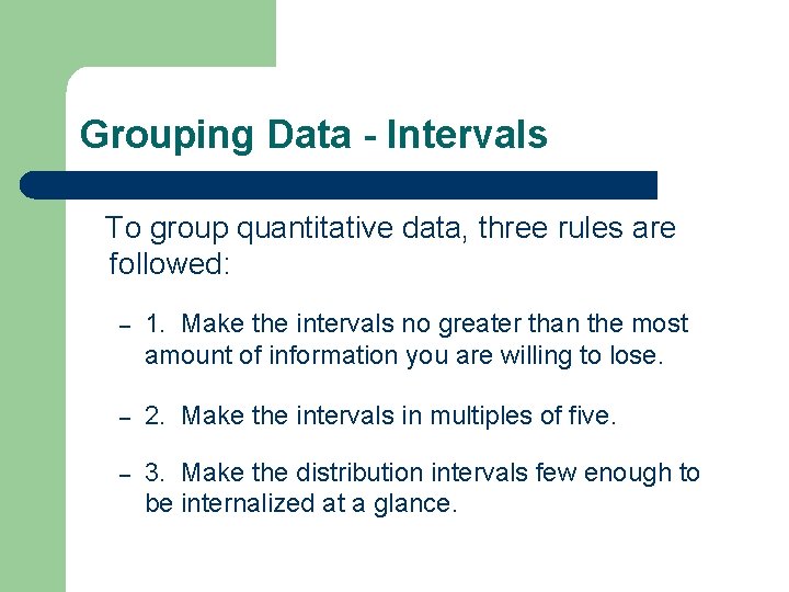
Grouping Data - Intervals To group quantitative data, three rules are followed: – 1. Make the intervals no greater than the most amount of information you are willing to lose. – 2. Make the intervals in multiples of five. – 3. Make the distribution intervals few enough to be internalized at a glance.

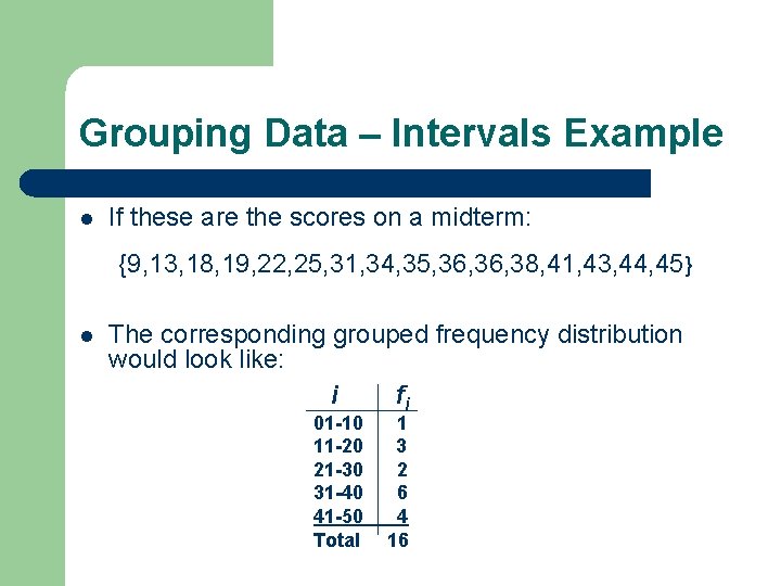
Grouping Data – Intervals Example l If these are the scores on a midterm: {9, 13, 18, 19, 22, 25, 31, 34, 35, 36, 38, 41, 43, 44, 45} l The corresponding grouped frequency distribution would look like: i fi 01 -10 11 -20 21 -30 31 -40 41 -50 Total 1 3 2 6 4 16

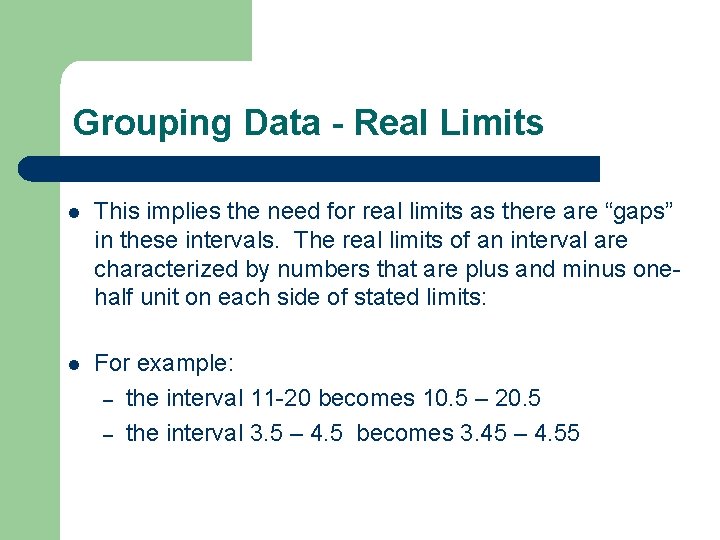
Grouping Data - Real Limits l This implies the need for real limits as there are “gaps” in these intervals. The real limits of an interval are characterized by numbers that are plus and minus onehalf unit on each side of stated limits: l For example: – the interval 11 -20 becomes 10. 5 – 20. 5 – the interval 3. 5 – 4. 5 becomes 3. 45 – 4. 55

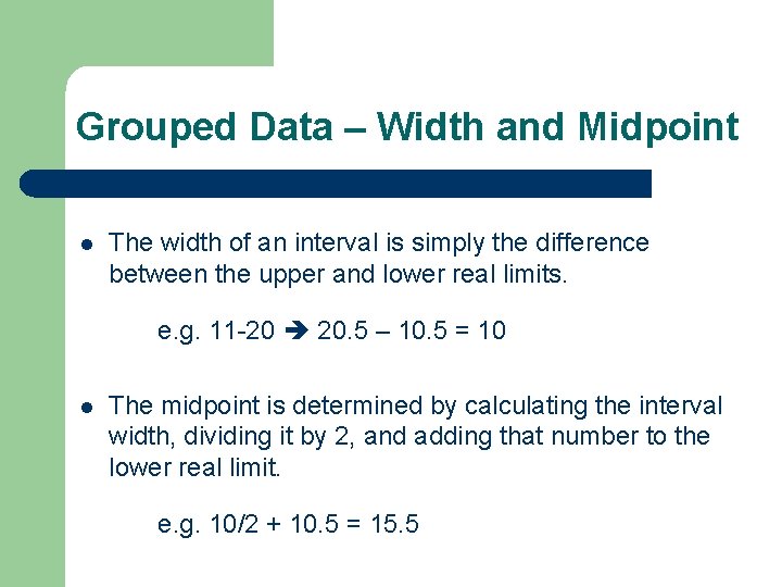
Grouped Data – Width and Midpoint l The width of an interval is simply the difference between the upper and lower real limits. e. g. 11 -20 20. 5 – 10. 5 = 10 l The midpoint is determined by calculating the interval width, dividing it by 2, and adding that number to the lower real limit. e. g. 10/2 + 10. 5 = 15. 5

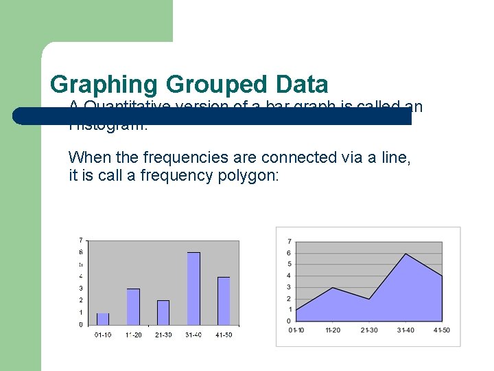
Graphing Grouped Data A Quantitative version of a bar graph is called an Histogram: When the frequencies are connected via a line, it is call a frequency polygon:

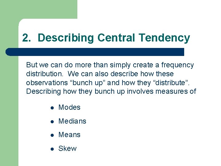
2. Describing Central Tendency But we can do more than simply create a frequency distribution. We can also describe how these observations “bunch up” and how they “distribute”. Describing how they bunch up involves measures of l Modes l Medians l Means l Skew

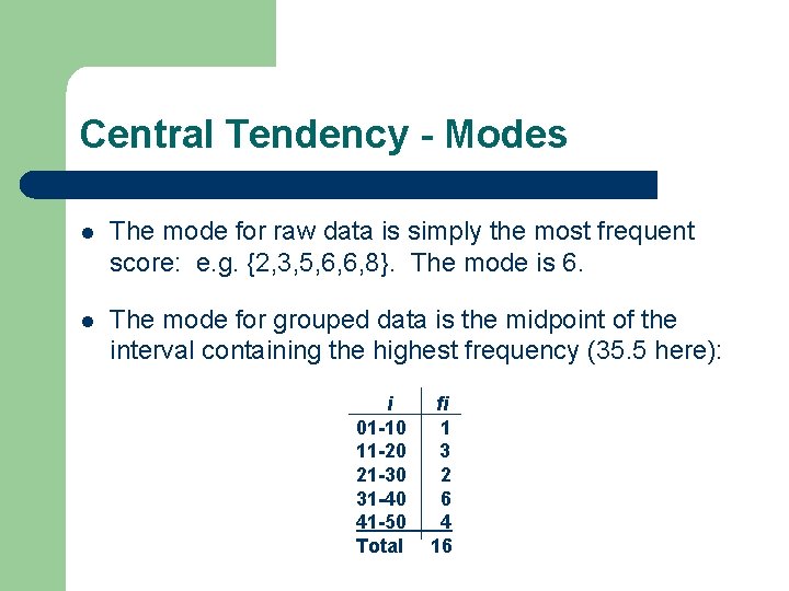
Central Tendency - Modes l The mode for raw data is simply the most frequent score: e. g. {2, 3, 5, 6, 6, 8}. The mode is 6. l The mode for grouped data is the midpoint of the interval containing the highest frequency (35. 5 here): i 01 -10 11 -20 21 -30 31 -40 41 -50 Total fi 1 3 2 6 4 16

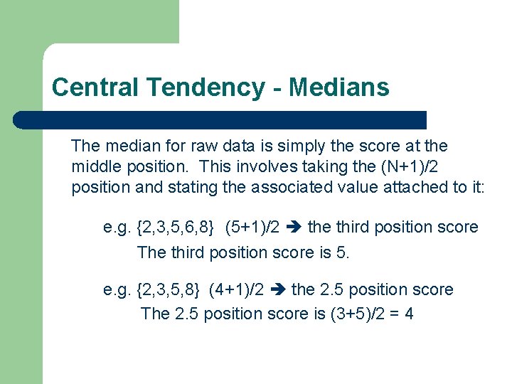
Central Tendency - Medians The median for raw data is simply the score at the middle position. This involves taking the (N+1)/2 position and stating the associated value attached to it: e. g. {2, 3, 5, 6, 8} (5+1)/2 the third position score The third position score is 5. e. g. {2, 3, 5, 8} (4+1)/2 the 2. 5 position score The 2. 5 position score is (3+5)/2 = 4

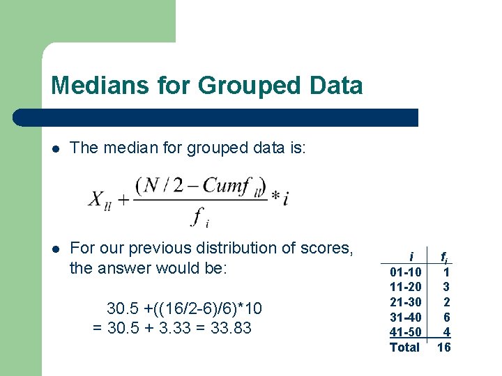
Medians for Grouped Data l The median for grouped data is: l For our previous distribution of scores, the answer would be: 30. 5 +((16/2 -6)/6)*10 = 30. 5 + 3. 33 = 33. 83 i 01 -10 11 -20 21 -30 31 -40 41 -50 Total fi 1 3 2 6 4 16

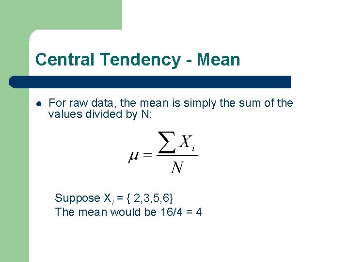
Central Tendency - Mean l For raw data, the mean is simply the sum of the values divided by N: Suppose Xi = { 2, 3, 5, 6} The mean would be 16/4 = 4

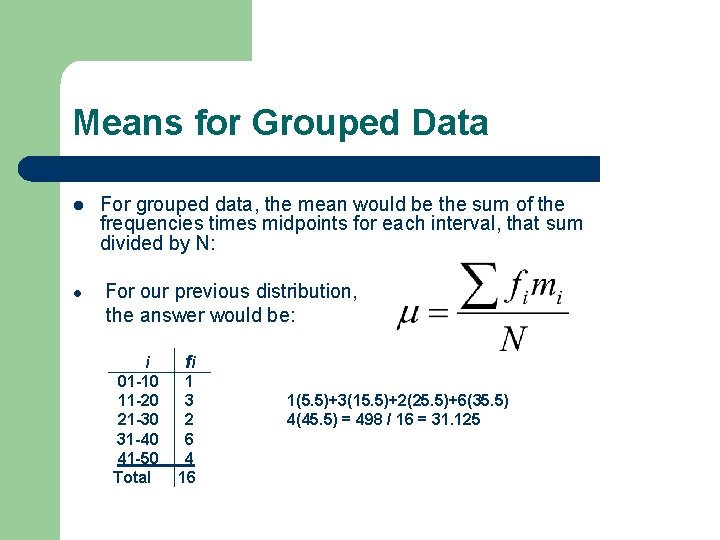
Means for Grouped Data l l For grouped data, the mean would be the sum of the frequencies times midpoints for each interval, that sum divided by N: For our previous distribution, the answer would be: i 01 -10 11 -20 21 -30 31 -40 41 -50 Total fi 1 3 2 6 4 16 1(5. 5)+3(15. 5)+2(25. 5)+6(35. 5) 4(45. 5) = 498 / 16 = 31. 125

3. Describing Variation l Range l Mean Deviation l Variance l Standard Scores (Z score)

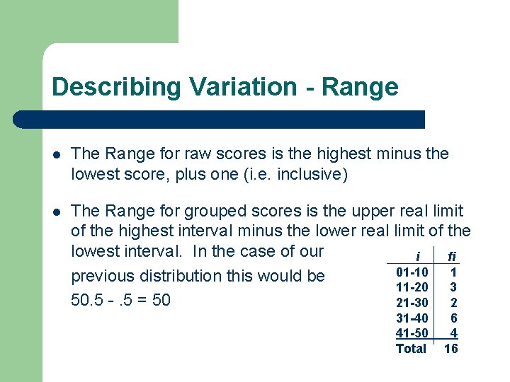
Describing Variation - Range l The Range for raw scores is the highest minus the lowest score, plus one (i. e. inclusive) l The Range for grouped scores is the upper real limit of the highest interval minus the lower real limit of the lowest interval. In the case of our i fi 01 -10 1 previous distribution this would be 11 -20 3 50. 5 -. 5 = 50 21 -30 2 31 -40 41 -50 Total 6 4 16

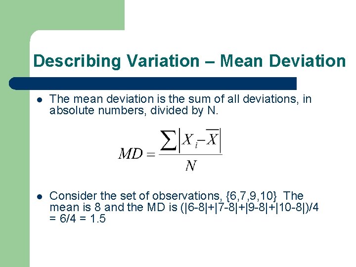
Describing Variation – Mean Deviation l The mean deviation is the sum of all deviations, in absolute numbers, divided by N. l Consider the set of observations, {6, 7, 9, 10} The mean is 8 and the MD is (|6 -8|+|7 -8|+|9 -8|+|10 -8|)/4 = 6/4 = 1. 5

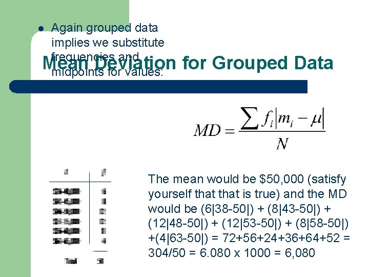
Again grouped data implies we substitute frequencies and Mean Deviation midpoints for values: l for Grouped Data The mean would be $50, 000 (satisfy yourself that is true) and the MD would be (6|38 -50|) + (8|43 -50|) + (12|48 -50|) + (12|53 -50|) + (8|58 -50|) +(4|63 -50|) = 72+56+24+36+64+52 = 304/50 = 6. 080 x 1000 = 6, 080

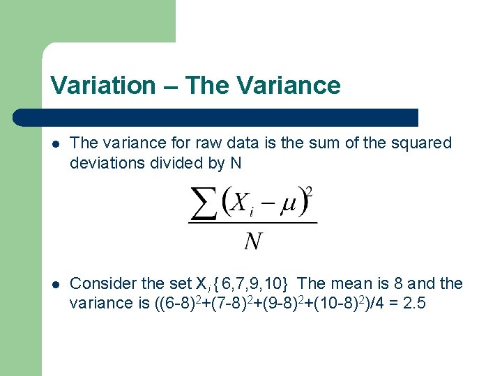
Variation – The Variance l The variance for raw data is the sum of the squared deviations divided by N l Consider the set Xi { 6, 7, 9, 10} The mean is 8 and the variance is ((6 -8)2+(7 -8)2+(9 -8)2+(10 -8)2)/4 = 2. 5

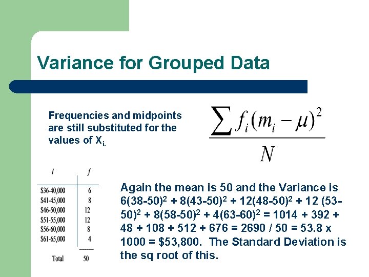
Variance for Grouped Data Frequencies and midpoints are still substituted for the values of Xi. Again the mean is 50 and the Variance is 6(38 -50)2 + 8(43 -50)2 + 12(48 -50)2 + 12 (5350)2 + 8(58 -50)2 + 4(63 -60)2 = 1014 + 392 + 48 + 108 + 512 + 676 = 2690 / 50 = 53. 8 x 1000 = $53, 800. The Standard Deviation is the sq root of this.

4. Covariance and Correlation l The Definition and Concept l The Formula l Proportional Reduction in Error and r 2

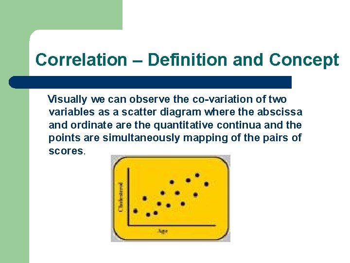
Correlation – Definition and Concept Visually we can observe the co-variation of two variables as a scatter diagram where the abscissa and ordinate are the quantitative continua and the points are simultaneously mapping of the pairs of scores.

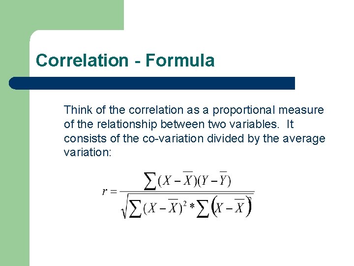
Correlation - Formula Think of the correlation as a proportional measure of the relationship between two variables. It consists of the co-variation divided by the average variation:

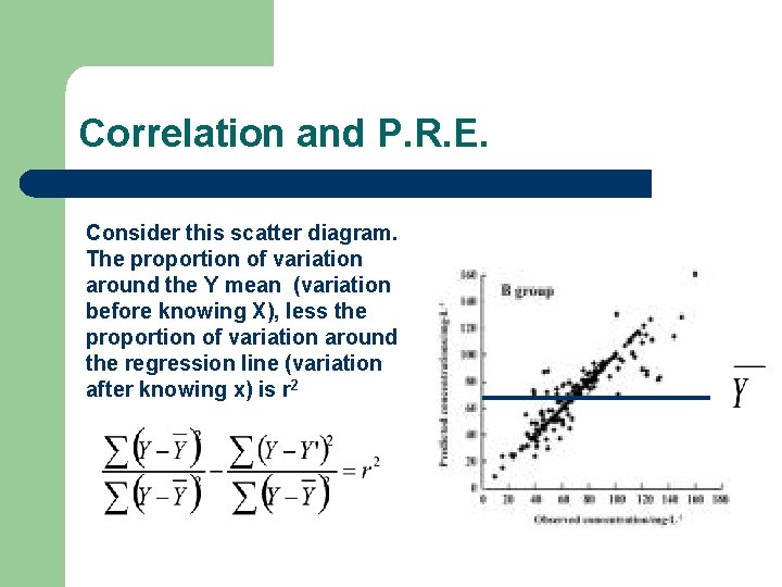
Correlation and P. R. E. Consider this scatter diagram. The proportion of variation around the Y mean (variation before knowing X), less the proportion of variation around the regression line (variation after knowing x) is r 2

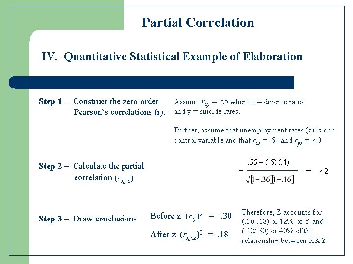
Partial Correlation IV. Quantitative Statistical Example of Elaboration Step 1 – Construct the zero order Pearson’s correlations (r). Assume rxy =. 55 where x = divorce rates and y = suicide rates. Further, assume that unemployment rates (z) is our control variable and that rxz =. 60 and ryz =. 40. 55 – (. 6) (. 4) Step 2 – Calculate the partial correlation (rxy. z) Step 3 – Draw conclusions = Before z (rxy)2 =. 30 After z (rxy. z)2 =. 18 =. 42 Therefore, Z accounts for (. 30 -. 18) or 12% of Y and (. 12/. 30) or 40% of the relationship between X&Y