Sociology 601 Class 8 September 24 2009 6

Sociology 601 Class 8: September 24, 2009 • 6. 6: Small-sample inference for a proportion • 7. 1: Large sample comparisons for two independent sample means. • 7. 2: Difference between two large sample proportions. 1

7. 1 Large sample comparisons for two independent means • So far, we have been making estimates and inferences about a single sample statistic • Now, we will begin making estimates and inferences for two sample statistics at once. – many real-life problems involve such comparisons – two-group problems often serve as a starting point for more involved statistics, as we shall see in this class. 2

Independent and dependent samples • Two independent random samples: – Two subsamples, each with a mean score for some other variable – example: Comparisons of work hours by race or sex – example: Comparison of earnings by marital status • Two dependent random samples: – Two observations are being compared for each “unit” in the sample – example: before-and-after measurements of the same person at two time points – example: earnings before and after marriage 3 – husband-wife differences

Comparison of two large-sample means for independent groups Hypothesis testing as we have done it so far: • Test statistic: z = (Ybar - o) / (s /SQRT(n)) • What can we do when we make inferences about a difference between population means ( 2 - 1)? – Treat one sample mean as if it were o ? – (NO: too much type I error) – Calculate a confidence interval for each sample mean and see if they overlap? – (NO: too much type II error) 4

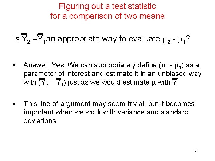
Figuring out a test statistic for a comparison of two means Is Y 2 –Y 1 an appropriate way to evaluate 2 - 1? • Answer: Yes. We can appropriately define ( 2 - 1) as a parameter of interest and estimate it in an unbiased way with (Y 2 – Y 1) just as we would estimate with Y. • This line of argument may seem trivial, but it becomes important when we work with variance and standard deviations. 5

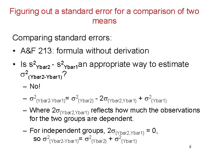
Figuring out a standard error for a comparison of two means Comparing standard errors: • A&F 213: formula without derivation • Is s 2 Ybar 2 - s 2 Ybar 1 an appropriate way to estimate 2(Ybar 2 -Ybar 1)? – No! – 2(Ybar 2 -Ybar 1)= 2(Ybar 2) - 2 (Ybar 2, Ybar 1) + 2(Ybar 1) – Where 2 (Ybar 2, Ybar 1) reflects how much the observations for the two groups are dependent. – For independent groups, 2 (Ybar 2, Ybar 1) = 0, so 2(Ybar 2 -Ybar 1)= 2(Ybar 2) + 2(Ybar 1) 6

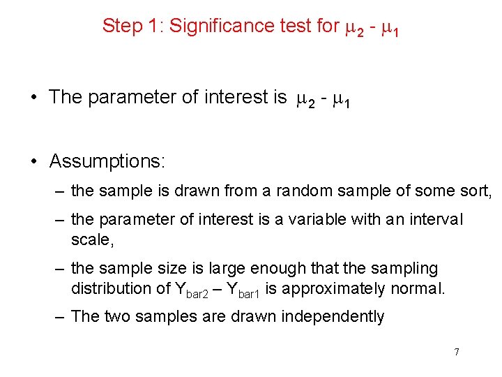
Step 1: Significance test for 2 - 1 • The parameter of interest is 2 - 1 • Assumptions: – the sample is drawn from a random sample of some sort, – the parameter of interest is a variable with an interval scale, – the sample size is large enough that the sampling distribution of Ybar 2 – Ybar 1 is approximately normal. – The two samples are drawn independently 7

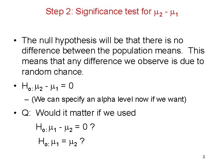
Step 2: Significance test for 2 - 1 • The null hypothesis will be that there is no difference between the population means. This means that any difference we observe is due to random chance. • Ho: 2 - 1 = 0 – (We can specify an alpha level now if we want) • Q: Would it matter if we used Ho: 1 - 2 = 0 ? Ho: 1 = 2 ? 8

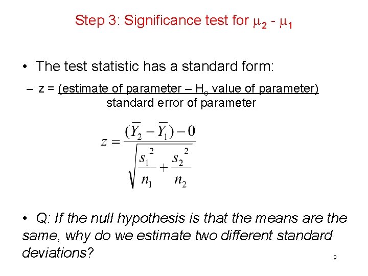
Step 3: Significance test for 2 - 1 • The test statistic has a standard form: – z = (estimate of parameter – Ho value of parameter) standard error of parameter • Q: If the null hypothesis is that the means are the same, why do we estimate two different standard deviations? 9

Step 4: Significance test for 2 - 1 P-value of calculated z: • Table A • Stata: display 2 * (1 – normal(z) ) • Stata: testi (no data, just parameters) • Stata: ttest (if data file in memory) 10

Step 5: Significance test for 2 - 1 Step 5: Conclusion. • Compare the p-value from step 4 to the alpha level in step 1. If p < α, reject H 0 If p ≥ α, do not reject H 0 • State a conclusion about the statistical significance of the test. • Briefly discuss the substantive importance of your findings. 11

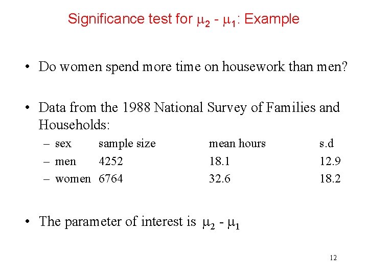
Significance test for 2 - 1: Example • Do women spend more time on housework than men? • Data from the 1988 National Survey of Families and Households: – sex sample size – men 4252 – women 6764 mean hours 18. 1 32. 6 s. d 12. 9 18. 2 • The parameter of interest is 2 - 1 12

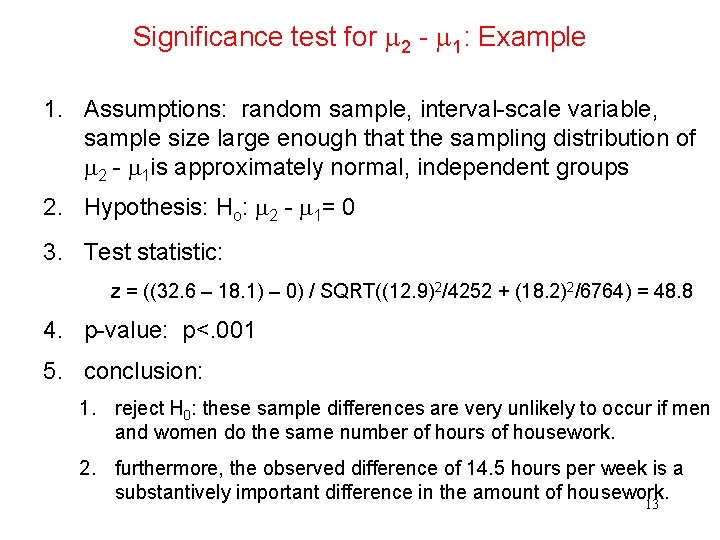
Significance test for 2 - 1: Example 1. Assumptions: random sample, interval-scale variable, sample size large enough that the sampling distribution of 2 - 1 is approximately normal, independent groups 2. Hypothesis: Ho: 2 - 1= 0 3. Test statistic: z = ((32. 6 – 18. 1) – 0) / SQRT((12. 9)2/4252 + (18. 2)2/6764) = 48. 8 4. p-value: p<. 001 5. conclusion: 1. reject H 0: these sample differences are very unlikely to occur if men and women do the same number of hours of housework. 2. furthermore, the observed difference of 14. 5 hours per week is a substantively important difference in the amount of housework. 13

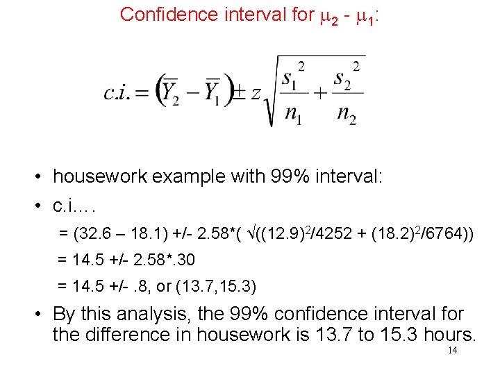
Confidence interval for 2 - 1: • housework example with 99% interval: • c. i…. = (32. 6 – 18. 1) +/- 2. 58*( √((12. 9)2/4252 + (18. 2)2/6764)) = 14. 5 +/- 2. 58*. 30 = 14. 5 +/-. 8, or (13. 7, 15. 3) • By this analysis, the 99% confidence interval for the difference in housework is 13. 7 to 15. 3 hours. 14

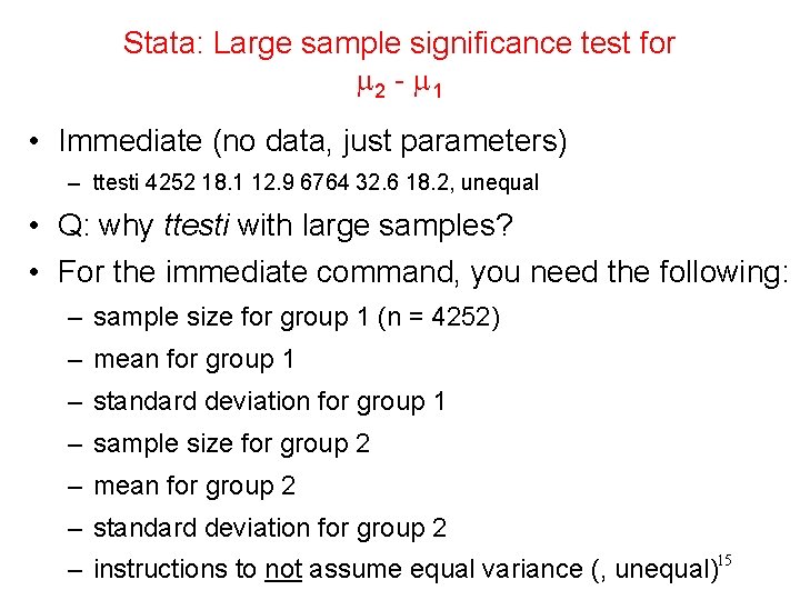
Stata: Large sample significance test for 2 - 1 • Immediate (no data, just parameters) – ttesti 4252 18. 1 12. 9 6764 32. 6 18. 2, unequal • Q: why ttesti with large samples? • For the immediate command, you need the following: – sample size for group 1 (n = 4252) – mean for group 1 – standard deviation for group 1 – sample size for group 2 – mean for group 2 – standard deviation for group 2 – instructions to not assume equal variance (, unequal)15

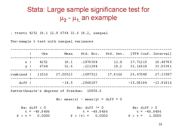
Stata: Large sample significance test for 2 - 1, an example. ttesti 4252 18. 1 12. 9 6764 32. 6 18. 2, unequal Two-sample t test with unequal variances ---------------------------------------| Obs Mean Std. Err. Std. Dev. [95% Conf. Interval] -----+----------------------------------x | 4252 18. 1. 1978304 12. 9 17. 71215 18. 48785 y | 6764 32. 6. 221294 18. 2 32. 16619 33. 03381 -----+----------------------------------combined | 11016 27. 00323. 1697512 17. 8166 26. 67049 27. 33597 -----+----------------------------------diff | -14. 5. 2968297 -15. 08184 -13. 91816 ---------------------------------------Satterthwaite's degrees of freedom: 10858. 6 Ho: mean(x) - mean(y) = diff = 0 Ha: diff < 0 t = -48. 8496 P < t = 0. 0000 Ha: diff != 0 t = -48. 8496 P > |t| = 0. 0000 Ha: diff > 0 t = -48. 8496 P > t = 1. 0000 16

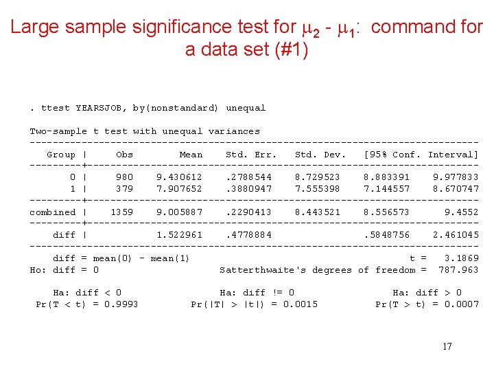
Large sample significance test for 2 - 1: command for a data set (#1). ttest YEARSJOB, by(nonstandard) unequal Two-sample t test with unequal variances ---------------------------------------Group | Obs Mean Std. Err. Std. Dev. [95% Conf. Interval] -----+----------------------------------0 | 980 9. 430612. 2788544 8. 729523 8. 883391 9. 977833 1 | 379 7. 907652. 3880947 7. 555398 7. 144557 8. 670747 -----+----------------------------------combined | 1359 9. 005887. 2290413 8. 443521 8. 556573 9. 4552 -----+----------------------------------diff | 1. 522961. 4778884. 5848756 2. 461045 ---------------------------------------diff = mean(0) - mean(1) t = 3. 1869 Ho: diff = 0 Satterthwaite's degrees of freedom = 787. 963 Ha: diff < 0 Pr(T < t) = 0. 9993 Ha: diff != 0 Pr(|T| > |t|) = 0. 0015 Ha: diff > 0 Pr(T > t) = 0. 0007 17

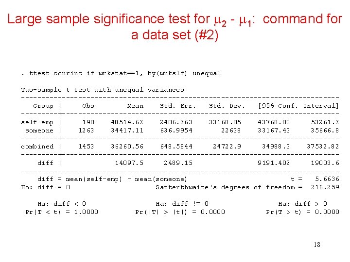
Large sample significance test for 2 - 1: command for a data set (#2). ttest conrinc if wrkstat==1, by(wrkslf) unequal Two-sample t test with unequal variances ---------------------------------------Group | Obs Mean Std. Err. Std. Dev. [95% Conf. Interval] -----+----------------------------------self-emp | 190 48514. 62 2406. 263 33168. 05 43768. 03 53261. 2 someone | 1263 34417. 11 636. 9954 22638 33167. 43 35666. 8 -----+----------------------------------combined | 1453 36260. 56 648. 5844 24722. 9 34988. 3 37532. 82 -----+----------------------------------diff | 14097. 5 2489. 15 9191. 402 19003. 6 ---------------------------------------diff = mean(self-emp) - mean(someone) t = 5. 6636 Ho: diff = 0 Satterthwaite's degrees of freedom = 216. 259 Ha: diff < 0 Pr(T < t) = 1. 0000 Ha: diff != 0 Pr(|T| > |t|) = 0. 0000 Ha: diff > 0 Pr(T > t) = 0. 0000 18

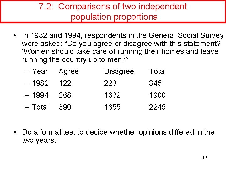
7. 2: Comparisons of two independent population proportions • In 1982 and 1994, respondents in the General Social Survey were asked: “Do you agree or disagree with this statement? ‘Women should take care of running their homes and leave running the country up to men. ’” – Year Agree Disagree Total – 1982 122 223 345 – 1994 268 1632 1900 – Total 390 1855 2245 • Do a formal test to decide whether opinions differed in the two years. 19

Step 1: Significance test for π2 - π1 • The parameter of interest is π2 - π1 • Assumptions: – the sample is drawn from a random sample of some sort, – the parameter of interest is a variable with an interval scale, – the sample size is large enough that the sampling distribution of Pihat 2 – Pihat 1 is approximately normal. – The two samples are drawn independently 20

Step 2: Significance test for π2 - π1 The null hypothesis will be that there is no difference between the population proportions. This means that any difference we observe is due to random chance. • Ho: π2 - π1 = 0 • (State an alpha here if you want to. ) 21

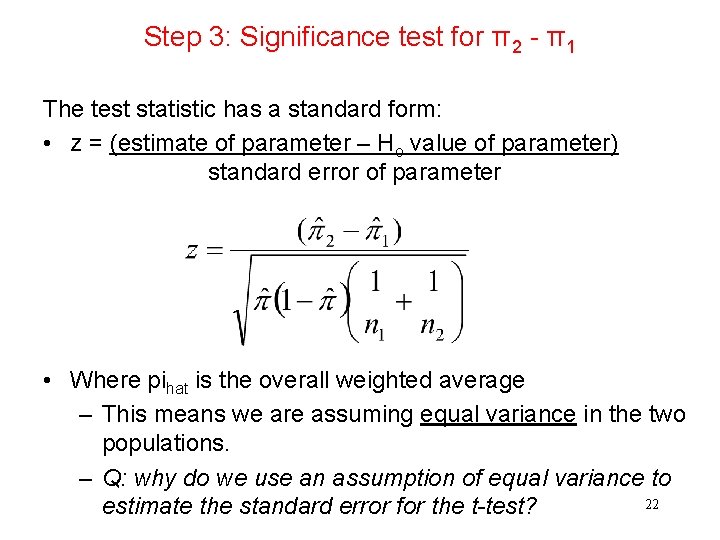
Step 3: Significance test for π2 - π1 The test statistic has a standard form: • z = (estimate of parameter – Ho value of parameter) standard error of parameter • Where pihat is the overall weighted average – This means we are assuming equal variance in the two populations. – Q: why do we use an assumption of equal variance to 22 estimate the standard error for the t-test?

Step 4: Significance test for π2 - π1 P-value of calculated z: • Table A, or • Stata: display 2 * (1 – normal(z) ), or • Stata: testi (no data, just parameters) • Stata: ttest (if data file in memory) 23

Step 5: Significance test for π2 - π1 Conclusion: • Compare the p-value from step 4 to the alpha level in step 1. If p < α, reject H 0 If p ≥ α, do not reject H 0 • State a conclusion about the statistical significance of the test. • Briefly discuss the substantive importance of your findings. 24

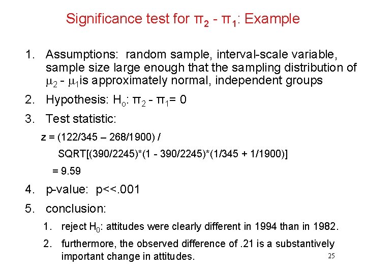
Significance test for π2 - π1: Example 1. Assumptions: random sample, interval-scale variable, sample size large enough that the sampling distribution of 2 - 1 is approximately normal, independent groups 2. Hypothesis: Ho: π2 - π1= 0 3. Test statistic: z = (122/345 – 268/1900) / SQRT[(390/2245)*(1 - 390/2245)*(1/345 + 1/1900)] = 9. 59 4. p-value: p<<. 001 5. conclusion: 1. reject H 0: attitudes were clearly different in 1994 than in 1982. 2. furthermore, the observed difference of. 21 is a substantively 25 important change in attitudes.

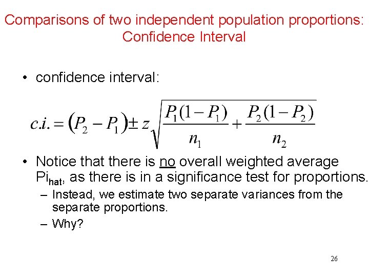
Comparisons of two independent population proportions: Confidence Interval • confidence interval: • Notice that there is no overall weighted average Pihat, as there is in a significance test for proportions. – Instead, we estimate two separate variances from the separate proportions. – Why? 26

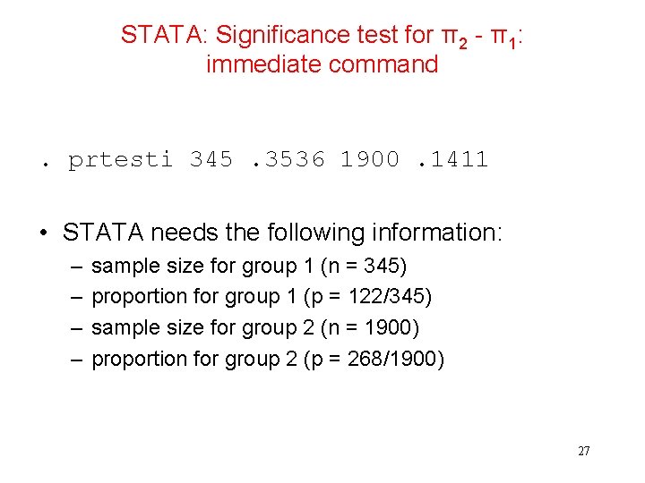
STATA: Significance test for π2 - π1: immediate command . prtesti 345. 3536 1900. 1411 • STATA needs the following information: – – sample size for group 1 (n = 345) proportion for group 1 (p = 122/345) sample size for group 2 (n = 1900) proportion for group 2 (p = 268/1900) 27

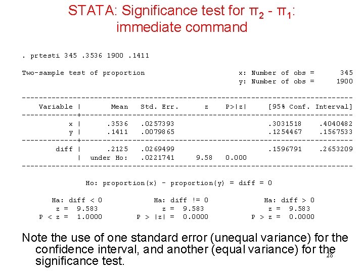
STATA: Significance test for π2 - π1: immediate command. prtesti 345. 3536 1900. 1411 Two-sample test of proportion x: Number of obs = y: Number of obs = 345 1900 ---------------------------------------Variable | Mean Std. Err. z P>|z| [95% Conf. Interval] -------+--------------------------------x |. 3536. 0257393. 3031518. 4040482 y |. 1411. 0079865. 1254467. 1567533 -------+--------------------------------diff |. 2125. 0269499. 1596791. 2653209 | under Ho: . 0221741 9. 58 0. 000 ---------------------------------------Ho: proportion(x) - proportion(y) = diff = 0 Ha: diff < 0 z = 9. 583 P < z = 1. 0000 Ha: diff != 0 z = 9. 583 P > |z| = 0. 0000 Ha: diff > 0 z = 9. 583 P > z = 0. 0000 Note the use of one standard error (unequal variance) for the confidence interval, and another (equal variance) for the 28 significance test.

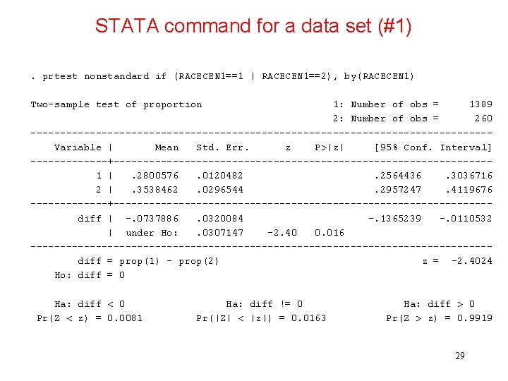
STATA command for a data set (#1). prtest nonstandard if (RACECEN 1==1 | RACECEN 1==2), by(RACECEN 1) Two-sample test of proportion 1: Number of obs = 1389 2: Number of obs = 260 ---------------------------------------Variable | Mean Std. Err. z P>|z| [95% Conf. Interval] -------+--------------------------------1 |. 2800576. 0120482. 2564436. 3036716 2 |. 3538462. 0296544. 2957247. 4119676 -------+--------------------------------diff | -. 0737886. 0320084 -. 1365239 -. 0110532 | under Ho: . 0307147 -2. 40 0. 016 ---------------------------------------diff = prop(1) - prop(2) z = -2. 4024 Ho: diff = 0 Ha: diff < 0 Pr(Z < z) = 0. 0081 Ha: diff != 0 Pr(|Z| < |z|) = 0. 0163 Ha: diff > 0 Pr(Z > z) = 0. 9919 29

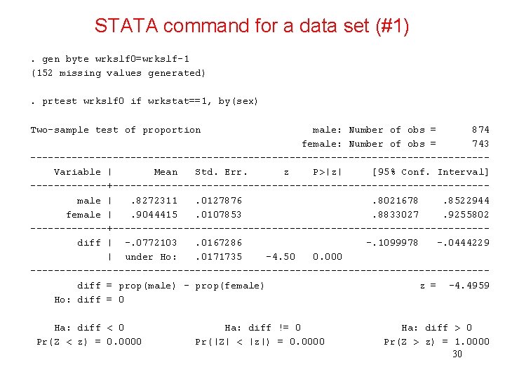
STATA command for a data set (#1). gen byte wrkslf 0=wrkslf-1 (152 missing values generated). prtest wrkslf 0 if wrkstat==1, by(sex) Two-sample test of proportion male: Number of obs = 874 female: Number of obs = 743 ---------------------------------------Variable | Mean Std. Err. z P>|z| [95% Conf. Interval] -------+--------------------------------male |. 8272311. 0127876. 8021678. 8522944 female |. 9044415. 0107853. 8833027. 9255802 -------+--------------------------------diff | -. 0772103. 0167286 -. 1099978 -. 0444229 | under Ho: . 0171735 -4. 50 0. 000 ---------------------------------------diff = prop(male) - prop(female) z = -4. 4959 Ho: diff = 0 Ha: diff < 0 Pr(Z < z) = 0. 0000 Ha: diff != 0 Pr(|Z| < |z|) = 0. 0000 Ha: diff > 0 Pr(Z > z) = 1. 0000 30