Social Network Theory Networked Life CSE 112 Spring
![The Binomial Distribution • The binomial distribution: – coin with Pr[heads] = p, flip The Binomial Distribution • The binomial distribution: – coin with Pr[heads] = p, flip](https://slidetodoc.com/presentation_image/3b67afc1ce2000db4fc01d9b5074412f/image-12.jpg)

- Slides: 47

Social Network Theory Networked Life CSE 112 Spring 2006 Prof. Michael Kearns

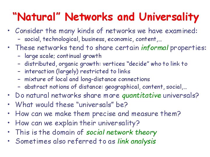
“Natural” Networks and Universality • Consider the many kinds of networks we have examined: – social, technological, business, economic, content, … • These networks tend to share certain informal properties: • • • – – – large scale; continual growth distributed, organic growth: vertices “decide” who to link to interaction (largely) restricted to links mixture of local and long-distance connections abstract notions of distance: geographical, content, social, … Do natural networks share more quantitative universals? What would these “universals” be? How can we make them precise and measure them? How can we explain their universality? This is the domain of social network theory Sometimes also referred to as link analysis

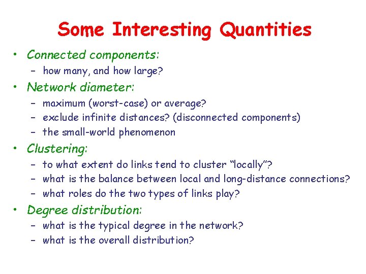
Some Interesting Quantities • Connected components: – how many, and how large? • Network diameter: – maximum (worst-case) or average? – exclude infinite distances? (disconnected components) – the small-world phenomenon • Clustering: – to what extent do links tend to cluster “locally”? – what is the balance between local and long-distance connections? – what roles do the two types of links play? • Degree distribution: – what is the typical degree in the network? – what is the overall distribution?

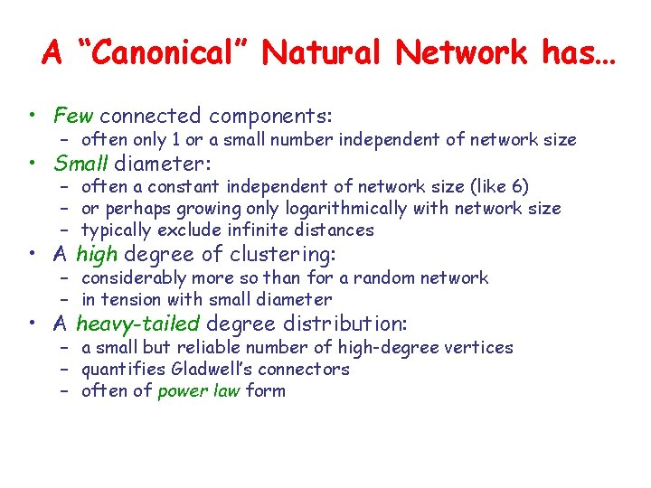
A “Canonical” Natural Network has… • Few connected components: – often only 1 or a small number independent of network size • Small diameter: – often a constant independent of network size (like 6) – or perhaps growing only logarithmically with network size – typically exclude infinite distances • A high degree of clustering: – considerably more so than for a random network – in tension with small diameter • A heavy-tailed degree distribution: – a small but reliable number of high-degree vertices – quantifies Gladwell’s connectors – often of power law form

Some Models of Network Generation • Random graphs (Erdos-Renyi models): – gives few components and small diameter – does not give high clustering and heavy-tailed degree distributions – is the mathematically most well-studied and understood model • Watts-Strogatz and related models: – give few components, small diameter and high clustering – does not give heavy-tailed degree distributions • Preferential attachment: – gives few components, small diameter and heavy-tailed distribution – does not give high clustering • Hierarchical networks: – few components, small diameter, high clustering, heavy-tailed • Affiliation networks: – models group-actor formation • Nothing “magic” about any of the measures or models

Approximate Roadmap • Examine a series of models of network generation – macroscopic properties they do and do not entail – pros and cons of each model • Examine some “real life” case studies • Study some dynamics issues (e. g. navigation) • Move into in-depth study of the web as network

Probabilistic Models of Networks • All of the network generation models we will study are probabilistic or statistical in nature • They can generate networks of any size • They often have various parameters that can be set: – size of network generated – average degree of a vertex – fraction of long-distance connections • The models generate a distribution over networks • Statements are always statistical in nature: – with high probability, diameter is small – on average, degree distribution has heavy tail • Thus, we’re going to need some basic statistics and probability theory

Statistics and Probability Theory: The Absolute, Bare-Minimum Essentials

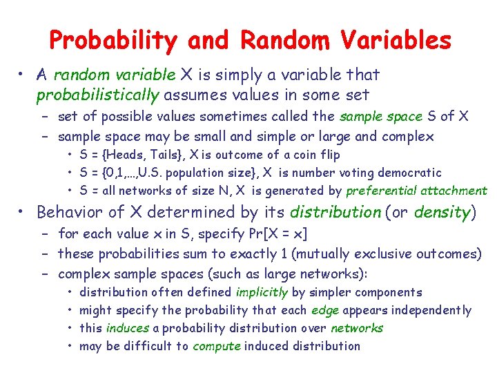
Probability and Random Variables • A random variable X is simply a variable that probabilistically assumes values in some set – set of possible values sometimes called the sample space S of X – sample space may be small and simple or large and complex • S = {Heads, Tails}, X is outcome of a coin flip • S = {0, 1, …, U. S. population size}, X is number voting democratic • S = all networks of size N, X is generated by preferential attachment • Behavior of X determined by its distribution (or density) – for each value x in S, specify Pr[X = x] – these probabilities sum to exactly 1 (mutually exclusive outcomes) – complex sample spaces (such as large networks): • • distribution often defined implicitly by simpler components might specify the probability that each edge appears independently this induces a probability distribution over networks may be difficult to compute induced distribution

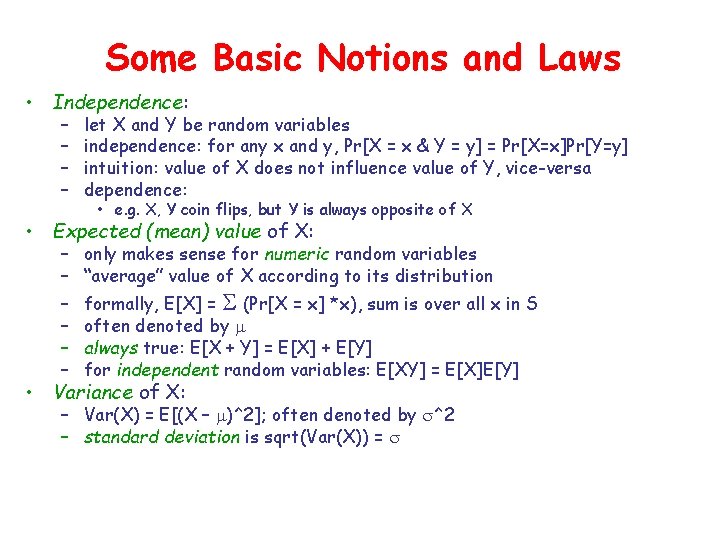
Some Basic Notions and Laws • Independence: – – let X and Y be random variables independence: for any x and y, Pr[X = x & Y = y] = Pr[X=x]Pr[Y=y] intuition: value of X does not influence value of Y, vice-versa dependence: • e. g. X, Y coin flips, but Y is always opposite of X • Expected (mean) value of X: – – – only makes sense for numeric random variables “average” value of X according to its distribution formally, E[X] = S (Pr[X = x] *x), sum is over all x in S often denoted by m always true: E[X + Y] = E[X] + E[Y] for independent random variables: E[XY] = E[X]E[Y] • Variance of X: – Var(X) = E[(X – m)^2]; often denoted by s^2 – standard deviation is sqrt(Var(X)) = s

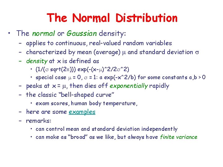
The Normal Distribution • The normal or Gaussian density: – applies to continuous, real-valued random variables – characterized by mean (average) m and standard deviation s – density at x is defined as • (1/(s sqrt(2 p))) exp(-(x-m)^2/2 s^2) • special case m = 0, s = 1: a exp(-x^2/b) for some constants a, b > 0 – peaks at x = m, then dies off exponentially rapidly – the classic “bell-shaped curve” • exam scores, human body temperature, – here are some examples – remarks: • can control mean and standard deviation independently • can make as “broad” as we like, but always have finite variance
![The Binomial Distribution The binomial distribution coin with Prheads p flip The Binomial Distribution • The binomial distribution: – coin with Pr[heads] = p, flip](https://slidetodoc.com/presentation_image/3b67afc1ce2000db4fc01d9b5074412f/image-12.jpg)
The Binomial Distribution • The binomial distribution: – coin with Pr[heads] = p, flip n times – probability of getting exactly k heads: • choose(n, k) p^k (1 -p)^(n-k) – for large n and p fixed: • approximated well by a normal with m = pn, s = sqrt(np(1 -p)) • s/m 0 as n grows • leads to strong large deviation bounds

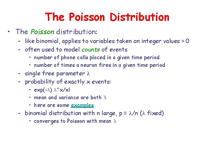
The Poisson Distribution • The Poisson distribution: – like binomial, applies to variables taken on integer values > 0 – often used to model counts of events • number of phone calls placed in a given time period • number of times a neuron fires in a given time period – single free parameter l – probability of exactly x events: • exp(-l) l^x/x! • mean and variance are both l • here are some examples – binomial distribution with n large, p = l/n (l fixed) • converges to Poisson with mean l

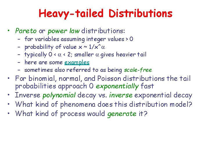
Heavy-tailed Distributions • Pareto or power law distributions: – – – for variables assuming integer values > 0 probability of value x ~ 1/x^a typically 0 < a < 2; smaller a gives heavier tail here are some examples sometimes also referred to as being scale-free • For binomial, normal, and Poisson distributions the tail probabilities approach 0 exponentially fast • Inverse polynomial decay vs. inverse exponential decay • What kind of phenomena does this distribution model? • What kind of process would generate it?

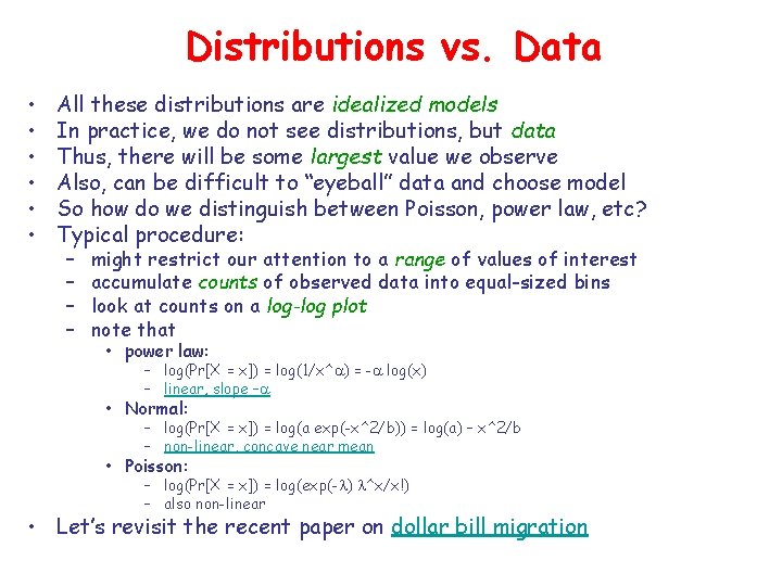
Distributions vs. Data • • • All these distributions are idealized models In practice, we do not see distributions, but data Thus, there will be some largest value we observe Also, can be difficult to “eyeball” data and choose model So how do we distinguish between Poisson, power law, etc? Typical procedure: – – might restrict our attention to a range of values of interest accumulate counts of observed data into equal-sized bins look at counts on a log-log plot note that • power law: – log(Pr[X = x]) = log(1/x^a) = -a log(x) – linear, slope –a • Normal: – log(Pr[X = x]) = log(a exp(-x^2/b)) = log(a) – x^2/b – non-linear, concave near mean • Poisson: – log(Pr[X = x]) = log(exp(-l) l^x/x!) – also non-linear • Let’s revisit the recent paper on dollar bill migration

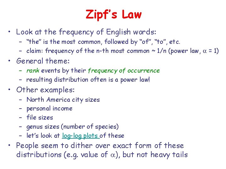
Zipf’s Law • Look at the frequency of English words: – “the” is the most common, followed by “of”, “to”, etc. – claim: frequency of the n-th most common ~ 1/n (power law, a = 1) • General theme: – rank events by their frequency of occurrence – resulting distribution often is a power law! • Other examples: – – – North America city sizes personal income file sizes genus sizes (number of species) let’s look at log-log plots of these • People seem to dither over exact form of these distributions (e. g. value of a), but not heavy tails

Models of Network Generation and Their Properties

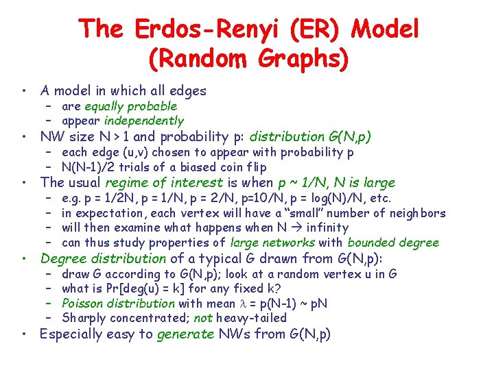
The Erdos-Renyi (ER) Model (Random Graphs) • A model in which all edges – are equally probable – appear independently • NW size N > 1 and probability p: distribution G(N, p) – each edge (u, v) chosen to appear with probability p – N(N-1)/2 trials of a biased coin flip • The usual regime of interest is when p ~ 1/N, N is large – – e. g. p = 1/2 N, p = 1/N, p = 2/N, p=10/N, p = log(N)/N, etc. in expectation, each vertex will have a “small” number of neighbors will then examine what happens when N infinity can thus study properties of large networks with bounded degree – – draw G according to G(N, p); look at a random vertex u in G what is Pr[deg(u) = k] for any fixed k? Poisson distribution with mean l = p(N-1) ~ p. N Sharply concentrated; not heavy-tailed • Degree distribution of a typical G drawn from G(N, p): • Especially easy to generate NWs from G(N, p)

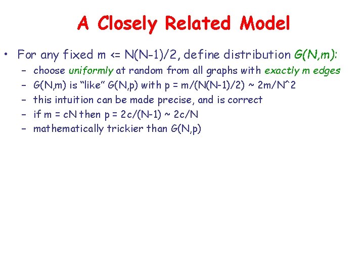
A Closely Related Model • For any fixed m <= N(N-1)/2, define distribution G(N, m): – – – choose uniformly at random from all graphs with exactly m edges G(N, m) is “like” G(N, p) with p = m/(N(N-1)/2) ~ 2 m/N^2 this intuition can be made precise, and is correct if m = c. N then p = 2 c/(N-1) ~ 2 c/N mathematically trickier than G(N, p)

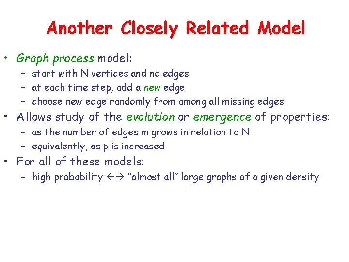
Another Closely Related Model • Graph process model: – start with N vertices and no edges – at each time step, add a new edge – choose new edge randomly from among all missing edges • Allows study of the evolution or emergence of properties: – as the number of edges m grows in relation to N – equivalently, as p is increased • For all of these models: – high probability “almost all” large graphs of a given density

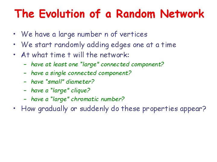
The Evolution of a Random Network • We have a large number n of vertices • We start randomly adding edges one at a time • At what time t will the network: – – – have at least one “large” connected component? have a single connected component? have “small” diameter? have a “large” clique? have a “large” chromatic number? • How gradually or suddenly do these properties appear?

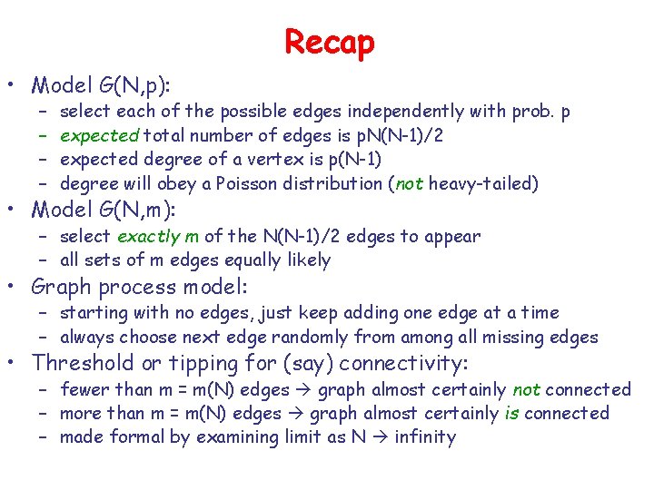
Recap • Model G(N, p): – – select each of the possible edges independently with prob. p expected total number of edges is p. N(N-1)/2 expected degree of a vertex is p(N-1) degree will obey a Poisson distribution (not heavy-tailed) • Model G(N, m): – select exactly m of the N(N-1)/2 edges to appear – all sets of m edges equally likely • Graph process model: – starting with no edges, just keep adding one edge at a time – always choose next edge randomly from among all missing edges • Threshold or tipping for (say) connectivity: – fewer than m = m(N) edges graph almost certainly not connected – more than m = m(N) edges graph almost certainly is connected – made formal by examining limit as N infinity

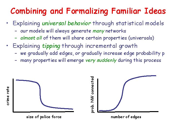
Combining and Formalizing Familiar Ideas • Explaining universal behavior through statistical models – our models will always generate many networks – almost all of them will share certain properties (universals) • Explaining tipping through incremental growth crime rate prob. NW connected – we gradually add edges, or gradually increase edge probability p – many properties will emerge very suddenly during this process size of police force number of edges

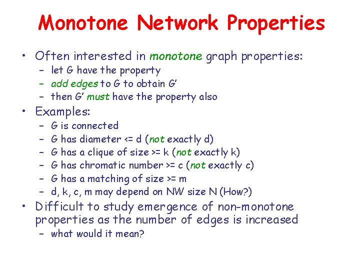
Monotone Network Properties • Often interested in monotone graph properties: – let G have the property – add edges to G to obtain G’ – then G’ must have the property also • Examples: – – – G is connected G has diameter <= d (not exactly d) G has a clique of size >= k (not exactly k) G has chromatic number >= c (not exactly c) G has a matching of size >= m d, k, c, m may depend on NW size N (How? ) • Difficult to study emergence of non-monotone properties as the number of edges is increased – what would it mean?

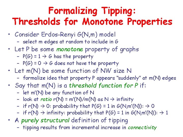
Formalizing Tipping: Thresholds for Monotone Properties • Consider Erdos-Renyi G(N, m) model – select m edges at random to include in G • Let P be some monotone property of graphs – P(G) = 1 G has the property – P(G) = 0 G does not have the property • Let m(N) be some function of NW size N – formalize idea that property P appears “suddenly” at m(N) edges • Say that m(N) is a threshold function for P if: – – let m’(N) be any function of N look at ratio r(N) = m’(N)/m(N) as N infinity if r(N) 0: probability that P(G) = 1 in G(N, m’(N)): 0 if r(N) infinity: probability that P(G) = 1 in G(N, m’(N)): 1 • A purely structural definition of tipping – tipping results from incremental increase in connectivity

So Which Properties Tip? • Just about all of them! • The following properties all have threshold functions: – – having a “giant component” being connected having a perfect matching (N even) having “small” diameter • Demo: look at the following progression – giant component connectivity small diameter – in graph process model (add one new edge at a time) – [example 1] [example 2] [example 3] [example 4] [example 5] • With remarkable consistency (N = 50): – giant component ~ 40 edges, connected ~ 100, small diameter ~ 180

Ever More Precise… • Connected component of size > N/2: – threshold function is m(N) = N (or p ~ 1/N) – note: full connectivity impossible • Fully connected: – threshold function is m(N) = (N/2)log(N) (or p ~ log(N)/N) – NW remains extremely sparse: only ~ log(N) edges per vertex • Small diameter: – threshold is m(N) ~ N^(3/2) for diameter 2 (or p ~ 2/sqrt(N)) – fraction of possible edges still ~ 2/sqrt(N) 0 – generate very small worlds

Other Tipping Points? • Perfect matchings – consider only even N – threshold function is m(N) = (N/2)log(N) (or p ~ log(N)/N) – same as for connectivity! • Cliques – k-clique threshold is m(N) = (1/2)N^(2 – 2/(k-1)) (p ~ 1/N^(2/k-1)) – edges appear immediately; triangles at N/2; etc. • Coloring – k colors required just as k-cliques appear

Erdos-Renyi Summary • A model in which all connections are equally likely – each of the N(N-1)/2 edges chosen randomly & independently • As we add edges, a precise sequence of events unfolds: – – • • graph acquires a giant component graph becomes connected graph acquires small diameter etc. Many properties appear very suddenly (tipping, thresholds) All statements are mathematically precise But is this how natural networks form? If not, which aspects are unrealistic? – maybe all edges are not equally likely!

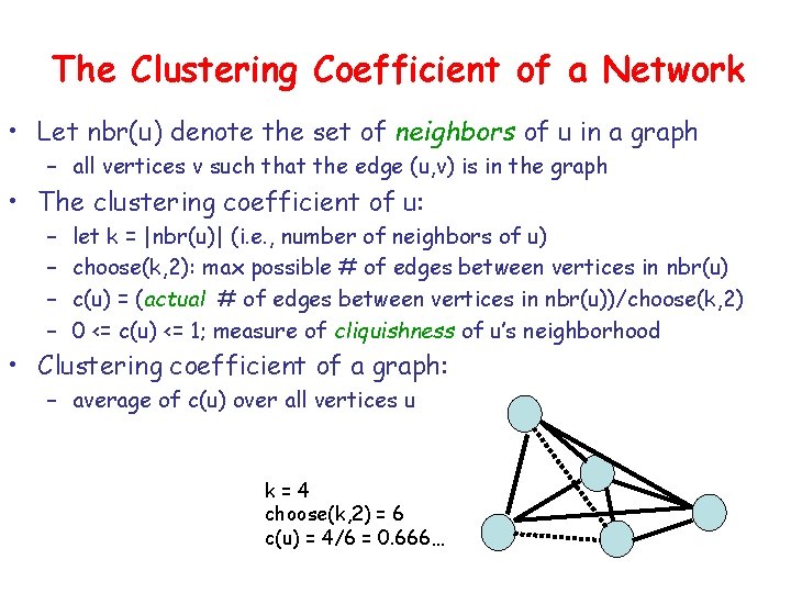
The Clustering Coefficient of a Network • Let nbr(u) denote the set of neighbors of u in a graph – all vertices v such that the edge (u, v) is in the graph • The clustering coefficient of u: – – let k = |nbr(u)| (i. e. , number of neighbors of u) choose(k, 2): max possible # of edges between vertices in nbr(u) c(u) = (actual # of edges between vertices in nbr(u))/choose(k, 2) 0 <= c(u) <= 1; measure of cliquishness of u’s neighborhood • Clustering coefficient of a graph: – average of c(u) over all vertices u k=4 choose(k, 2) = 6 c(u) = 4/6 = 0. 666…

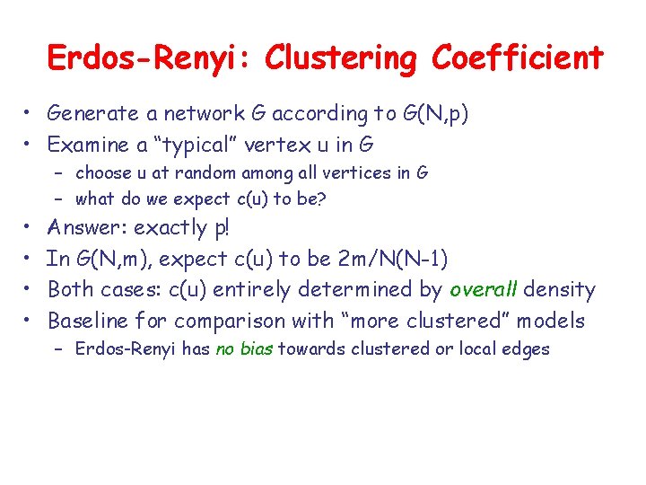
Erdos-Renyi: Clustering Coefficient • Generate a network G according to G(N, p) • Examine a “typical” vertex u in G – choose u at random among all vertices in G – what do we expect c(u) to be? • • Answer: exactly p! In G(N, m), expect c(u) to be 2 m/N(N-1) Both cases: c(u) entirely determined by overall density Baseline for comparison with “more clustered” models – Erdos-Renyi has no bias towards clustered or local edges

Caveman and Solaria • Erdos-Renyi: – sharing a common neighbor makes two vertices no more likely to be directly connected than two very “distant” vertices – every edge appears entirely independently of existing structure • But in many settings, the opposite is true: – you tend to meet new friends through your old friends – two web pages pointing to a third might share a topic – two companies selling goods to a third are in related industries • Watts’ Caveman world: – overall density of edges is low – but two vertices with a common neighbor are likely connected • Watts’ Solaria world – overall density of edges low; no special bias towards local edges – “like” Erdos-Renyi

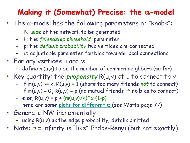
Making it (Somewhat) Precise: the a-model • The a-model has the following parameters or “knobs”: – N: size of the network to be generated – k: the friendship threshold parameter – p: the default probability two vertices are connected – a: adjustable parameter for bias towards local connections • For any vertices u and v: – define m(u, v) to be the number of common neighbors (so far) • Key quantity: the propensity R(u, v) of u to connect to v – – if m(u, v) >= k, R(u, v) = 1 (share too many friends not to connect) if m(u, v) = 0, R(u, v) = p (no mutual friends no bias to connect) else, R(u, v) = p + (m(u, v)/k)^a (1 -p) here are some plots for different a (see Watts page 77) • Generate NW incrementally – using R(u, v) as the edge probability; details omitted • Note: a = infinity is “like” Erdos-Renyi (but not exactly)

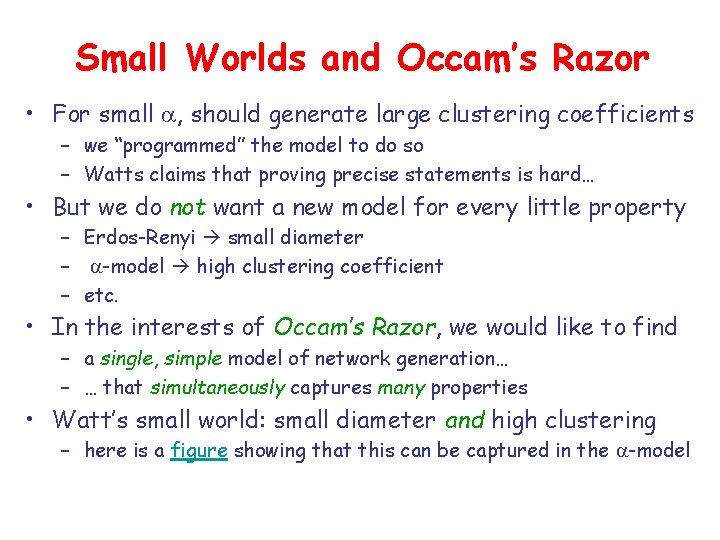
Small Worlds and Occam’s Razor • For small a, should generate large clustering coefficients – we “programmed” the model to do so – Watts claims that proving precise statements is hard… • But we do not want a new model for every little property – Erdos-Renyi small diameter – a-model high clustering coefficient – etc. • In the interests of Occam’s Razor, we would like to find – a single, simple model of network generation… – … that simultaneously captures many properties • Watt’s small world: small diameter and high clustering – here is a figure showing that this can be captured in the a-model

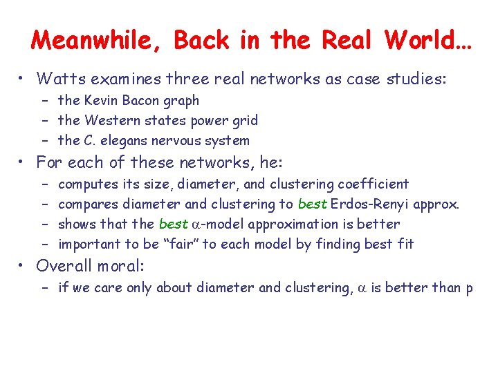
Meanwhile, Back in the Real World… • Watts examines three real networks as case studies: – the Kevin Bacon graph – the Western states power grid – the C. elegans nervous system • For each of these networks, he: – – computes its size, diameter, and clustering coefficient compares diameter and clustering to best Erdos-Renyi approx. shows that the best a-model approximation is better important to be “fair” to each model by finding best fit • Overall moral: – if we care only about diameter and clustering, a is better than p

Case 1: Kevin Bacon Graph • Vertices: actors and actresses • Edge between u and v if they appeared in a film together • Here is the data

Case 2: Western States Power Grid • Vertices: power stations in Western U. S. • Edges: high-voltage power transmission lines • Here is the network and data

Case 3: C. Elegans Nervous System • Vertices: neurons in the C. elegans worm • Edges: axons/synapses between neurons • Here is the network and data

Two More Examples • M. Newman on scientific collaboration networks – coauthorship networks in several distinct communities – differences in degrees (papers per author) – empirical verification of • giant components • small diameter (mean distance) • high clustering coefficient • Alberich et al. on the Marvel Universe – purely fictional social network – two characters linked if they appeared together in an issue – “empirical” verification of • heavy-tailed distribution of degrees (issues and characters) • giant component • rather small clustering coefficient

One More (Structural) Property… • A properly tuned a-model can simultaneously explain – small diameter – high clustering coefficient • But what about heavy-tailed degree distributions? – a-model and simple variants will not explain this – intuitively, no “bias” towards large degree evolves – all vertices are created equal • Can concoct many bad generative models to explain – generate NW according to Erdos-Renyi, reject if tails not heavy – describe fixed NWs with heavy tails • all connected to v 1; N/2 connected to v 2; etc. • not clear we can get a precise power law • not modeling variation – why would the world evolve this way? • As always, we want a “natural” model

Preferential Attachment • Start with (say) two vertices connected by an edge • For i = 3 to N: – for each 1 <= j < i, let d(j) be degree of vertex j (so far) – let Z = S d(j) (sum of all degrees so far) – add new vertex i with k edges back to {1, …, i-1}: • i is connected back to j with probability d(j)/Z • Vertices j with high degree are likely to get more links! • “Rich get richer” • Natural model for many processes: – hyperlinks on the web – new business and social contacts – transportation networks • Generates a power law distribution of degrees – exponent depends on value of k

Two Out of Three Isn’t Bad… • Preferential attachment explains – heavy-tailed degree distributions – small diameter (~log(N), via “hubs”) • Will not generate high clustering coefficient – no bias towards local connectivity, but towards hubs • Can we simultaneously capture all three properties? – probably, but we’ll stop here – soon there will be a fourth property anyway…

Search and Navigation

Finding Short Paths • Milgram’s experiment, Columbia Small Worlds, a-model… – all emphasize existence of short paths between pairs • How do individuals find short paths – in an incremental, next-step fashion – using purely local information about the NW and location of target • This is not a structural question, but an algorithmic one – statics vs. dynamics • Navigability may impose additional restrictions on model! • Briefly investigate two alternatives: – variation on the a-model – a “social identity” model

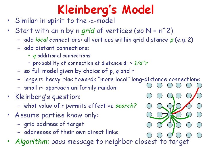
Kleinberg’s Model • Similar in spirit to the a-model • Start with an n by n grid of vertices (so N = n^2) – add local connections: all vertices within grid distance p (e. g. 2) – add distant connections: • q additional connections • probability of connection at distance d: ~ 1/d^r – so full model given by choice of p, q and r – large r: heavy bias towards “more local” long-distance connections – small r: approach uniformly random • Kleinberg’s question: – what value of r permits effective search? • Assume parties know only: – grid address of target – addresses of their own direct links • Algorithm: pass message to neighbor closest to target

Kleinberg’s Result • Intuition: – if r is too large (strong local bias), then “long-distance” connections never help much; short paths may not even exist – if r is too small (no local bias), we may quickly get close to the target; but then we’ll have to use local links to finish • think of a transport system with only long-haul jets or donkey carts – effective search requires a delicate mixture of link distances • The result (informally): – – r = 2 is the only value that permits rapid navigation (~log(N) steps) any other value of r will result in time ~ N^c for 0 < c <= 1 a critical value phenomenon contrast with 1/d^(1. 59) from recent dollar bill migration paper • Note: locality of information crucial to this argument – centralized algorithm may compute short paths at large r – can recognize when “backwards” steps are beneficial

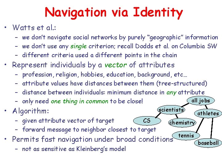
Navigation via Identity • Watts et al. : – we don’t navigate social networks by purely “geographic” information – we don’t use any single criterion; recall Dodds et al. on Columbia SW – different criteria used a different points in the chain • Represent individuals by a vector of attributes – – profession, religion, hobbies, education, background, etc… attribute values have distances between them (tree-structured) distance between individuals: minimum distance in any attribute all jobs only need one thing in common to be close! • Algorithm: – given attribute vector of target CS – forward message to neighbor closest to target scientists chemistry • Permits fast navigation under broad conditions – not as sensitive as Kleinberg’s model athletes tennis baseball