Soc 3306 a Multiple Regression Testing a Model

Soc 3306 a Multiple Regression Testing a Model and Interpreting Coefficients

Assumptions for Multiple Regression Random sample n Distribution of y is relatively normal n ¨ Check n histogram for DV Standard deviation of y is constant for each value of x ¨ Check scatterplots (Figure 1)

Problems to Watch For… Violation of assumptions, especially normality of DV and heteroscedasticity (Figure 1) n Simpson’s Paradox (Figure 3) n Multicollinearity (Figure 1 and 2) n

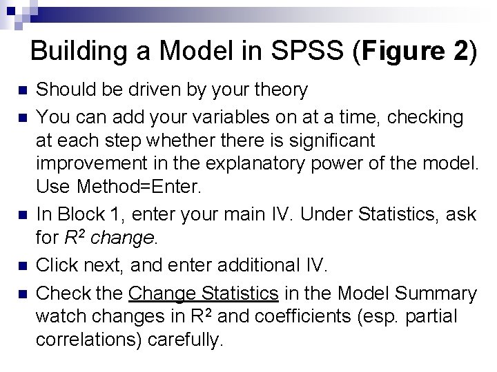
Building a Model in SPSS (Figure 2) n n n Should be driven by your theory You can add your variables on at a time, checking at each step whethere is significant improvement in the explanatory power of the model. Use Method=Enter. In Block 1, enter your main IV. Under Statistics, ask for R 2 change. Click next, and enter additional IV. Check the Change Statistics in the Model Summary watch changes in R 2 and coefficients (esp. partial correlations) carefully.

Multiple Correlation R (Figure 2) Measures correlation of all IV’s with DV n Is the correlation of y values with the predicted y values n Always positive (between 0 and +1) n

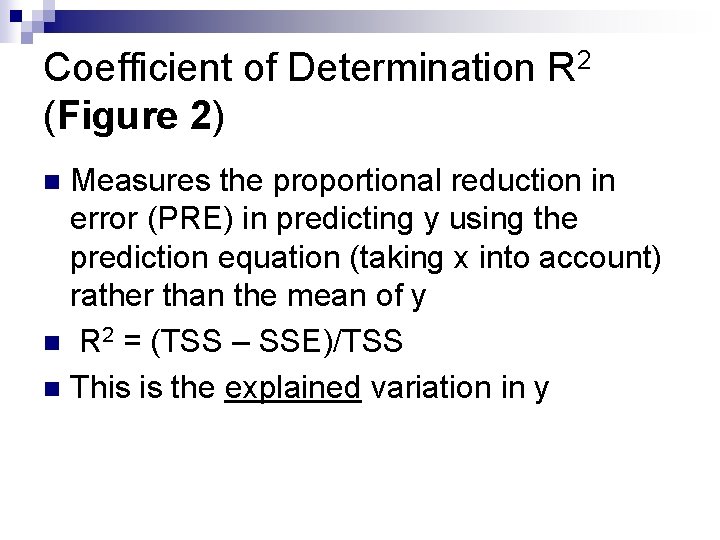
Coefficient of Determination R 2 (Figure 2) Measures the proportional reduction in error (PRE) in predicting y using the prediction equation (taking x into account) rather than the mean of y n R 2 = (TSS – SSE)/TSS n This is the explained variation in y n

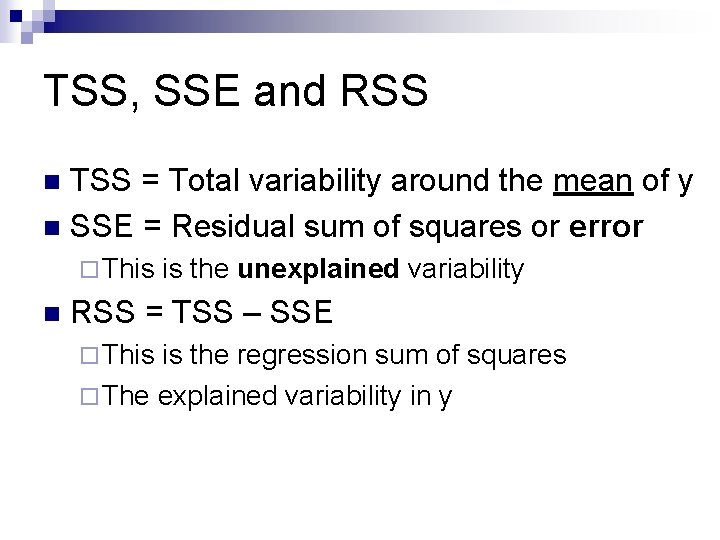
TSS, SSE and RSS TSS = Total variability around the mean of y n SSE = Residual sum of squares or error n ¨ This n is the unexplained variability RSS = TSS – SSE ¨ This is the regression sum of squares ¨ The explained variability in y

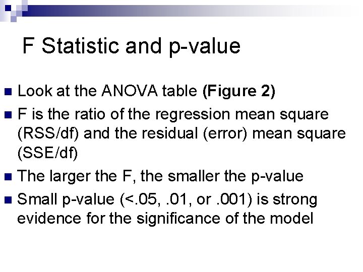
F Statistic and p-value Look at the ANOVA table (Figure 2) n F is the ratio of the regression mean square (RSS/df) and the residual (error) mean square (SSE/df) n The larger the F, the smaller the p-value n Small p-value (<. 05, . 01, or. 001) is strong evidence for the significance of the model n

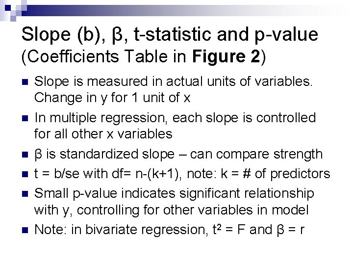
Slope (b), β, t-statistic and p-value (Coefficients Table in Figure 2) n n n Slope is measured in actual units of variables. Change in y for 1 unit of x In multiple regression, each slope is controlled for all other x variables β is standardized slope – can compare strength t = b/se with df= n-(k+1), note: k = # of predictors Small p-value indicates significant relationship with y, controlling for other variables in model Note: in bivariate regression, t 2 = F and β = r

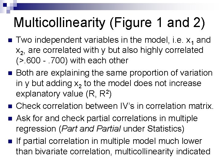
Multicollinearity (Figure 1 and 2) n n n Two independent variables in the model, i. e. x 1 and x 2, are correlated with y but also highly correlated (>. 600 -. 700) with each other Both are explaining the same proportion of variation in y but adding x 2 to the model does not increase explanatory value (R, R 2) Check correlation between IV’s in correlation matrix. Ask for and check partial correlations in multiple regression (Part and Partial under Statistics) If partial correlation in multiple model much lower than bivariate correlation, multicollinearity indicated

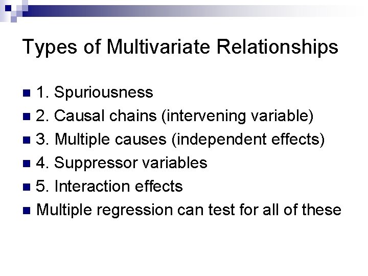
Types of Multivariate Relationships 1. Spuriousness n 2. Causal chains (intervening variable) n 3. Multiple causes (independent effects) n 4. Suppressor variables n 5. Interaction effects n Multiple regression can test for all of these n

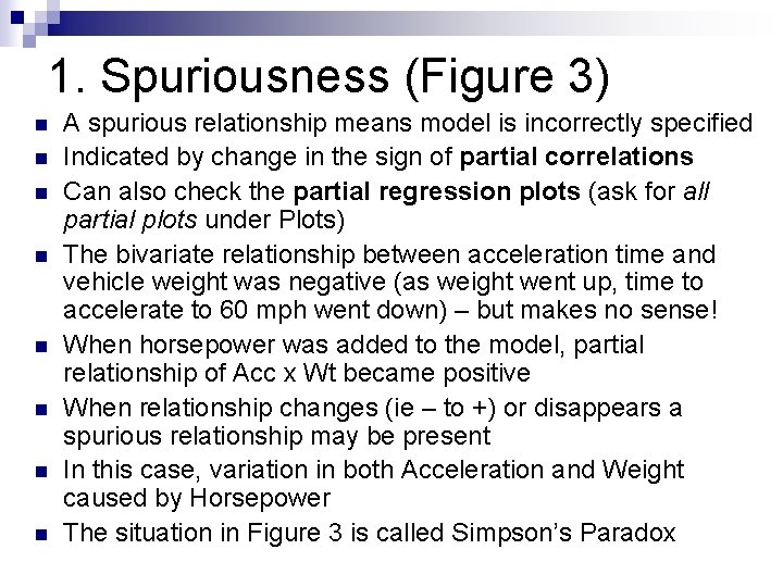
1. Spuriousness (Figure 3) n n n n A spurious relationship means model is incorrectly specified Indicated by change in the sign of partial correlations Can also check the partial regression plots (ask for all partial plots under Plots) The bivariate relationship between acceleration time and vehicle weight was negative (as weight went up, time to accelerate to 60 mph went down) – but makes no sense! When horsepower was added to the model, partial relationship of Acc x Wt became positive When relationship changes (ie – to +) or disappears a spurious relationship may be present In this case, variation in both Acceleration and Weight caused by Horsepower The situation in Figure 3 is called Simpson’s Paradox

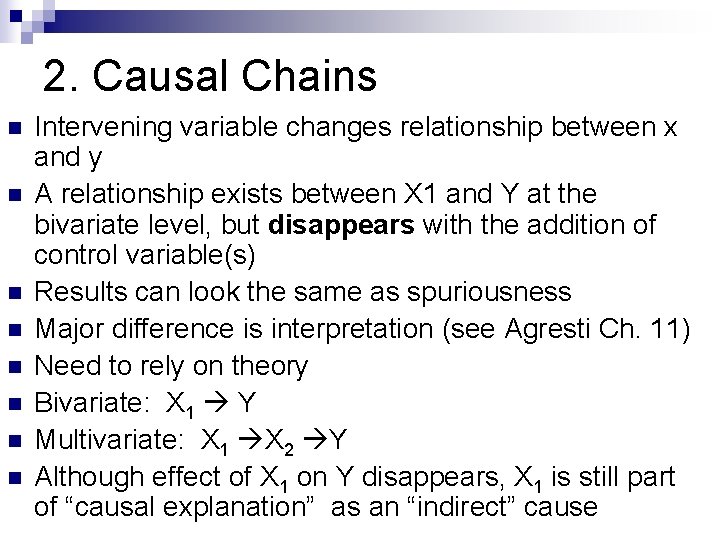
2. Causal Chains n n n n Intervening variable changes relationship between x and y A relationship exists between X 1 and Y at the bivariate level, but disappears with the addition of control variable(s) Results can look the same as spuriousness Major difference is interpretation (see Agresti Ch. 11) Need to rely on theory Bivariate: X 1 Y Multivariate: X 1 X 2 Y Although effect of X 1 on Y disappears, X 1 is still part of “causal explanation” as an “indirect” cause

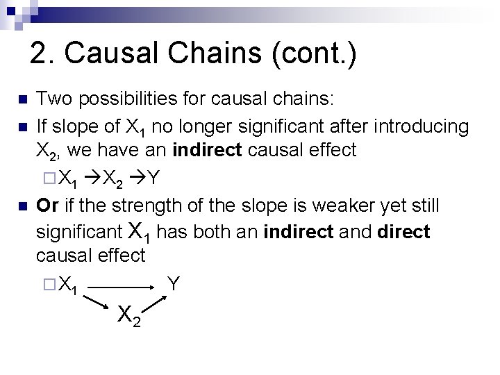
2. Causal Chains (cont. ) n n n Two possibilities for causal chains: If slope of X 1 no longer significant after introducing X 2, we have an indirect causal effect ¨ X 1 X 2 Y Or if the strength of the slope is weaker yet still significant X 1 has both an indirect and direct causal effect ¨ X 1 Y X 2

3. Multiple Causes Y (DV) has multiple causes n Independent variables have relatively separate effects on the dependent variable n Introduction of controls does little to change bivariate correlations and the bivariate slopes stay similar n Compare bivariate to partial correlations in multiple model and compare slopes in the bivariate and multiple models n

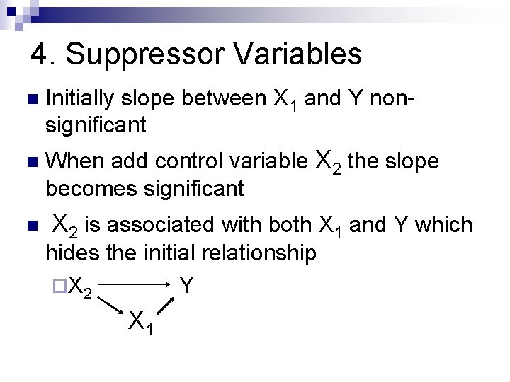
4. Suppressor Variables n Initially slope between X 1 and Y nonsignificant n When add control variable X 2 the slope becomes significant n X 2 is associated with both X 1 and Y which hides the initial relationship ¨X 2 Y X 1

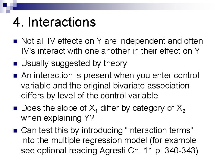
4. Interactions n n n Not all IV effects on Y are independent and often IV’s interact with one another in their effect on Y Usually suggested by theory An interaction is present when you enter control variable and the original bivariate association differs by level of the control variable Does the slope of X 1 differ by category of X 2 when explaining Y? Can test this by introducing “interaction terms” into the multiple regression model (for example see optional reading Agresti Ch. 11 p. 340 -343)

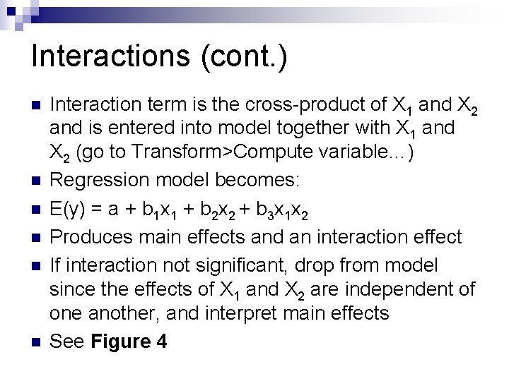
Interactions (cont. ) n n n Interaction term is the cross-product of X 1 and X 2 and is entered into model together with X 1 and X 2 (go to Transform>Compute variable…) Regression model becomes: E(y) = a + b 1 x 1 + b 2 x 2 + b 3 x 1 x 2 Produces main effects and an interaction effect If interaction not significant, drop from model since the effects of X 1 and X 2 are independent of one another, and interpret main effects See Figure 4

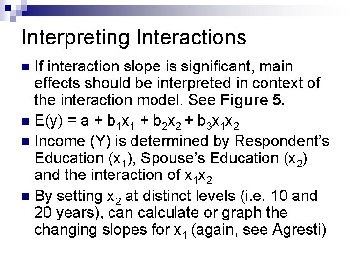
Interpreting Interactions If interaction slope is significant, main effects should be interpreted in context of the interaction model. See Figure 5. n E(y) = a + b 1 x 1 + b 2 x 2 + b 3 x 1 x 2 n Income (Y) is determined by Respondent’s Education (x 1), Spouse’s Education (x 2) and the interaction of x 1 x 2 n By setting x 2 at distinct levels (i. e. 10 and 20 years), can calculate or graph the changing slopes for x 1 (again, see Agresti) n

A Few Tips for SPSS Mini 6 n n n Review the relevant powerpoint slides and accompanying handouts Read assignment over carefully before starting. When creating your model, build your model carefully one block at a time. Watch for spurious relationships. Revise model if needed. Drop any unnecessary variables (i. e. evidence of multicollinearity or new variables that do not appreciably increase R 2. ) Keep your model simple. Aim for good explanatory value with the least variables possible.