SMRs PMRs and Survival Measures Principles of Epidemiology

SMRs, PMRs and Survival Measures Principles of Epidemiology Lecture 3 Dona Schneider, Ph. D, MPH, FACE

REVIEW: Adjusted Rates are Created Through Standardization n Standardization: n The process by which you derive a summary figure to compare health outcomes of groups n The process can be used for mortality, natality, or morbidity data Epidemiology (Schneider)

Standardization Examples n Direct Method requires n Age-specific rates in the sample population n The age of each case n The population-at-risk for each age group in the sample n Age structure (percentage of cases in each age group) of a standard population n Summary figure is an AGE-ADJUSTED RATE Epidemiology (Schneider)

Standardization: Age Adjustment (cont. ) n Indirect method requires n Age structure of the sample population at risk n Total cases in the sample population (not ages of cases) n Age-specific rates for a standard population n Summary figure is a STANDARDIZED MORTALITY RATIO (SMR) Epidemiology (Schneider)

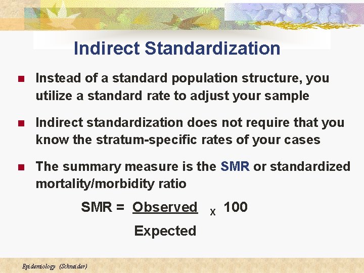
Indirect Standardization n Instead of a standard population structure, you utilize a standard rate to adjust your sample n Indirect standardization does not require that you know the stratum-specific rates of your cases n The summary measure is the SMR or standardized mortality/morbidity ratio SMR = Observed Expected Epidemiology (Schneider) X 100

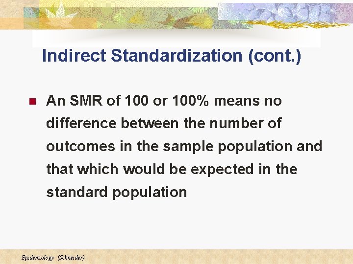
Indirect Standardization (cont. ) n An SMR of 100 or 100% means no difference between the number of outcomes in the sample population and that which would be expected in the standard population Epidemiology (Schneider)

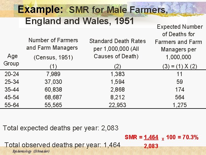
Example: SMR for Male Farmers, England Wales, 1951 (Census, 1951) Standard Death Rates per 1, 000 (All Causes of Death) Expected Number of Deaths for Farmers and Farm Managers per 1, 000 (1) 7, 989 37, 030 60, 838 68, 687 55, 565 (2) 1, 383 1, 594 2, 868 8, 212 22, 953 (3) = (1) X (2) 11 59 174 564 1, 275 Number of Farmers and Farm Managers Age Group 20 -24 25 -34 35 -44 45 -54 55 -64 Total expected deaths per year: 2, 083 SMR = 1, 464 Total observed deaths per year: 1, 464 Epidemiology (Schneider) 2, 083 X 100 = 70. 3%

In 1951, male farmers in England Wales had a mortality rate 30 percent lower than the comparably-aged general population.

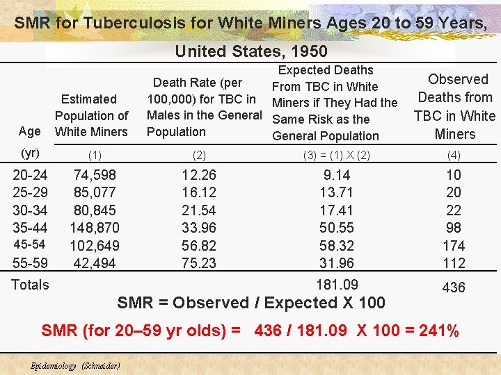
SMR for Tuberculosis for White Miners Ages 20 to 59 Years, United States, 1950 Age Estimated Population of White Miners Expected Deaths Death Rate (per From TBC in White 100, 000) for TBC in Miners if They Had the Males in the General Same Risk as the Population General Population Observed Deaths from TBC in White Miners (yr) (1) (2) (3) = (1) X (2) (4) 20 -24 25 -29 30 -34 35 -44 74, 598 85, 077 80, 845 148, 870 102, 649 42, 494 12. 26 16. 12 21. 54 33. 96 56. 82 75. 23 9. 14 13. 71 17. 41 50. 55 58. 32 31. 96 10 20 22 98 174 112 181. 09 436 45 -54 55 -59 Totals SMR = Observed / Expected X 100 SMR (for 20– 59 yr olds) = 436 / 181. 09 X 100 = 241% Epidemiology (Schneider)

In the United States in 1950, white miners ages 20 to 59 years died of tuberculosis almost 2. 5 times as often as comparably-aged males in the general population Epidemiology (Schneider)

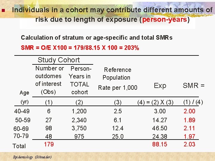
n Individuals in a cohort may contribute different amounts of risk due to length of exposure (person-years) Calculation of stratum or age-specific and total SMRs SMR = O/E X 100 = 179/88. 15 X 100 = 203% Study Cohort Number or Personoutdomes Years in of interest TOTAL (Obs) cohort Age (yr) 40 -49 50 -59 60 -69 70 -79 Total Reference Population Rate per 1, 000 (1) 6 (2) 1, 200 (3) 2. 5 27 98 48 179 2, 340 3, 750 975 6. 1 12. 4 25. 0 Epidemiology (Schneider) Exp (4) = (2) X (3) 3. 00 14. 27 46. 50 24. 38 88. 15 SMR = (1) / (4) 2. 00 1. 89 2. 11 1. 97 2. 03

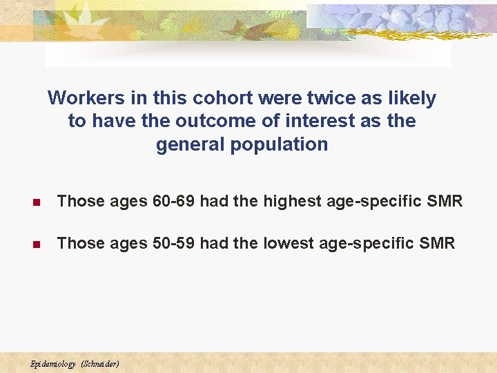
Workers in this cohort were twice as likely to have the outcome of interest as the general population n Those ages 60 -69 had the highest age-specific SMR n Those ages 50 -59 had the lowest age-specific SMR Epidemiology (Schneider)

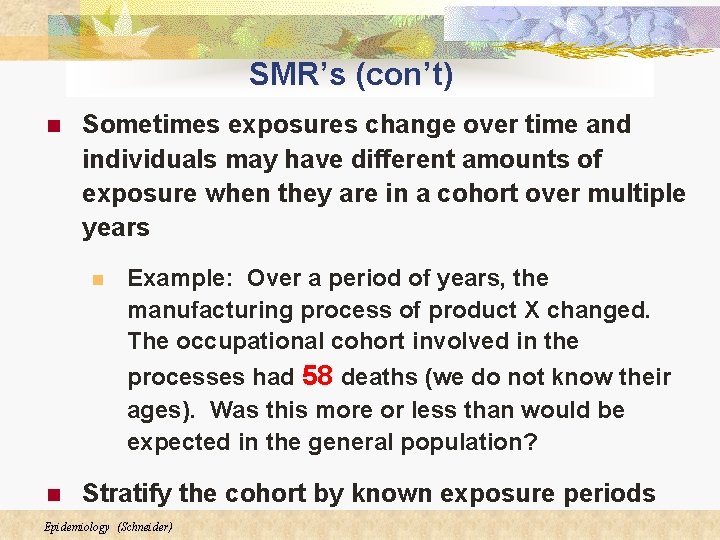
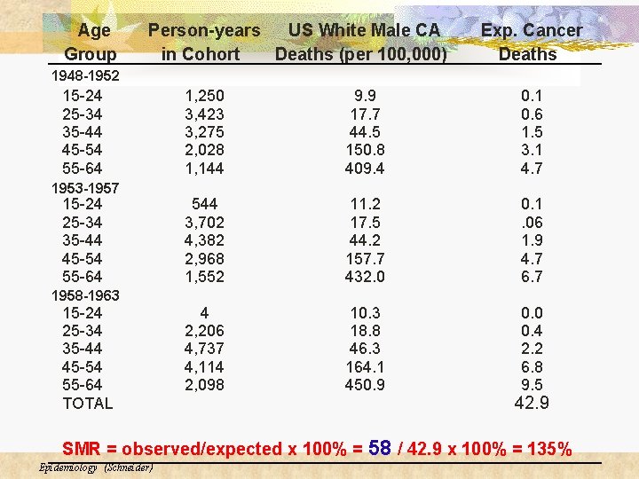
SMR’s (con’t) n Sometimes exposures change over time and individuals may have different amounts of exposure when they are in a cohort over multiple years n n Example: Over a period of years, the manufacturing process of product X changed. The occupational cohort involved in the processes had 58 deaths (we do not know their ages). Was this more or less than would be expected in the general population? Stratify the cohort by known exposure periods Epidemiology (Schneider)

Age Group Person-years US White Male CA in Cohort Deaths (per 100, 000) Exp. Cancer Deaths 1948 -1952 15 -24 25 -34 35 -44 45 -54 55 -64 1953 -1957 15 -24 25 -34 35 -44 45 -54 55 -64 1958 -1963 15 -24 25 -34 35 -44 45 -54 55 -64 TOTAL 1, 250 3, 423 3, 275 2, 028 1, 144 9. 9 17. 7 44. 5 150. 8 409. 4 0. 1 0. 6 1. 5 3. 1 4. 7 544 3, 702 4, 382 2, 968 1, 552 11. 2 17. 5 44. 2 157. 7 432. 0 0. 1. 06 1. 9 4. 7 6. 7 4 2, 206 4, 737 4, 114 2, 098 10. 3 18. 8 46. 3 164. 1 450. 9 0. 0 0. 4 2. 2 6. 8 9. 5 42. 9 SMR = observed/expected x 100% = 58 / 42. 9 x 100% = 135% Epidemiology (Schneider)

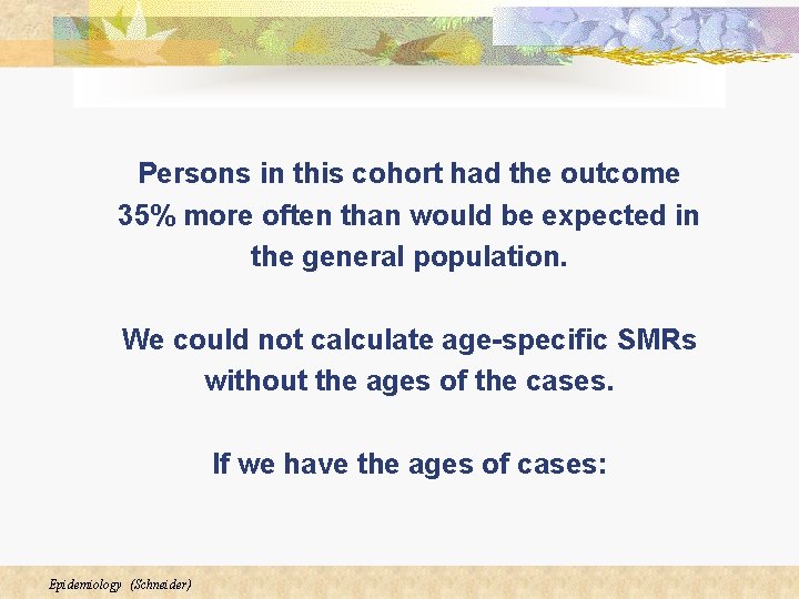
Persons in this cohort had the outcome 35% more often than would be expected in the general population. We could not calculate age-specific SMRs without the ages of the cases. If we have the ages of cases: Epidemiology (Schneider)

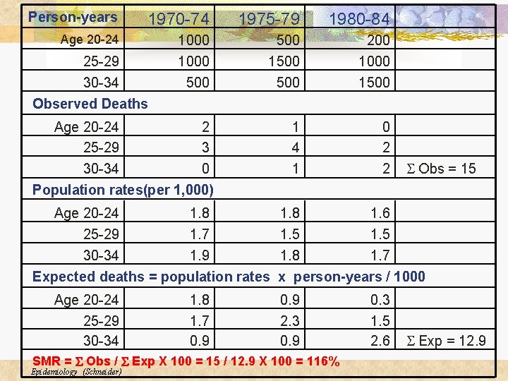
Person-years 1970 -74 1975 -79 1980 -84 Age 20 -24 1000 500 1500 200 1000 1500 Age 20 -24 2 25 -29 3 30 -34 0 Population rates(per 1, 000) 1 4 1 0 2 2 25 -29 30 -34 Observed Deaths Age 20 -24 1. 8 25 -29 1. 7 30 -34 1. 9 Expected deaths = population rates Age 20 -24 25 -29 30 -34 1. 8 1. 7 0. 9 1. 8 1. 6 1. 5 1. 8 1. 7 x person-years / 1000 0. 9 2. 3 0. 9 SMR = S Obs / S Exp X 100 = 15 / 12. 9 X 100 = 116% Epidemiology (Schneider) S Obs = 15 0. 3 1. 5 2. 6 S Exp = 12. 9

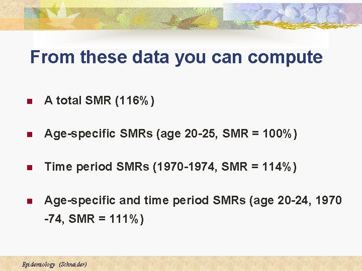
From these data you can compute n A total SMR (116%) n Age-specific SMRs (age 20 -25, SMR = 100%) n Time period SMRs (1970 -1974, SMR = 114%) n Age-specific and time period SMRs (age 20 -24, 1970 -74, SMR = 111%) Epidemiology (Schneider)

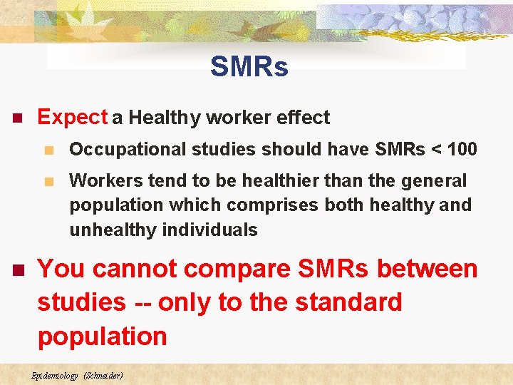
SMRs n n Expect a Healthy worker effect n Occupational studies should have SMRs < 100 n Workers tend to be healthier than the general population which comprises both healthy and unhealthy individuals You cannot compare SMRs between studies -- only to the standard population Epidemiology (Schneider)

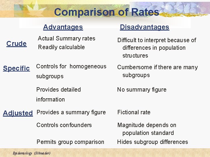
Comparison of Rates Advantages Crude Actual Summary rates Readily calculable Specific Controls for homogeneous Disadvantages Difficult to interpret because of differences in population structures subgroups Cumbersome if there are many subgroups Provides detailed No summary figure information Adjusted Provides a summary figure Fictional rate Controls confounders Magnitude depends on population standard Permits group comparison Hides subgroup differences Epidemiology (Schneider)

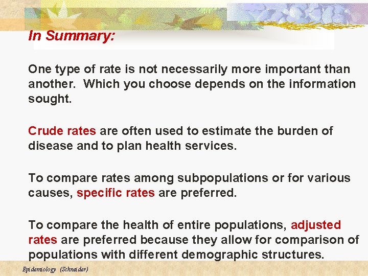
In Summary: One type of rate is not necessarily more important than another. Which you choose depends on the information sought. Crude rates are often used to estimate the burden of disease and to plan health services. To compare rates among subpopulations or for various causes, specific rates are preferred. To compare the health of entire populations, adjusted rates are preferred because they allow for comparison of populations with different demographic structures. Epidemiology (Schneider)

CDC Wonder http: //wonder. cdc. gov/ Epidemiology (Schneider)

Additional Outcome Measures n Proportionate Mortality Ratio n Proportionate Mortality Rate n Case Fatality Rate n Years of Potential Life Lost n Measures of Survival Epidemiology (Schneider)

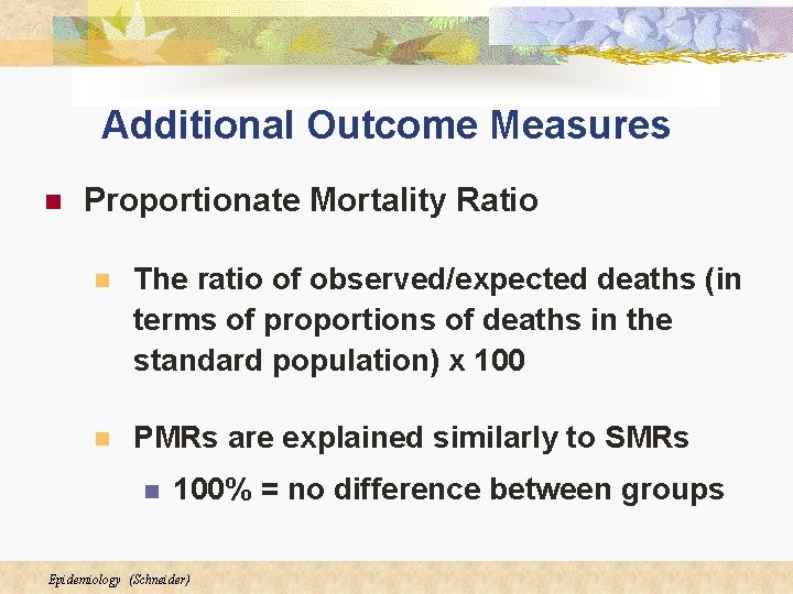
Additional Outcome Measures n Proportionate Mortality Ratio n The ratio of observed/expected deaths (in terms of proportions of deaths in the standard population) x 100 n PMRs are explained similarly to SMRs n 100% = no difference between groups Epidemiology (Schneider)

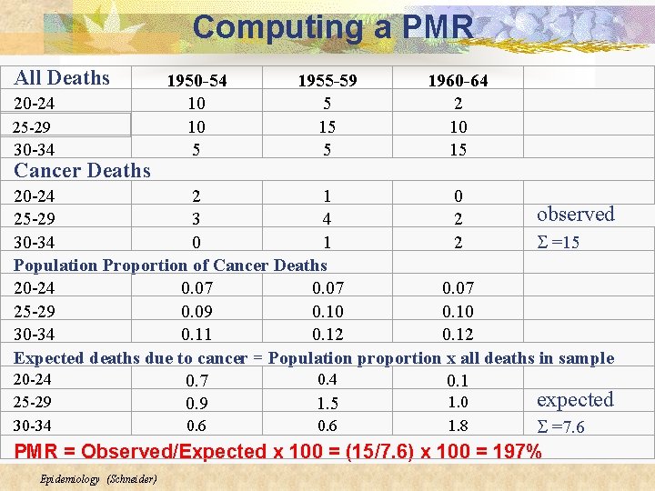
Computing a PMR All Deaths 20 -24 25 -29 30 -34 Cancer Deaths 1950 -54 10 10 5 1955 -59 5 15 5 1960 -64 2 10 15 20 -24 2 1 0 observed 25 -29 3 4 2 30 -34 0 1 2 S =15 Population Proportion of Cancer Deaths 20 -24 0. 07 25 -29 0. 09 0. 10 30 -34 0. 11 0. 12 Expected deaths due to cancer = Population proportion x all deaths in sample 20 -24 0. 7 0. 1 expected 25 -29 1. 0 0. 9 1. 5 30 -34 0. 6 1. 8 S =7. 6 PMR = Observed/Expected x 100 = (15/7. 6) x 100 = 197% Epidemiology (Schneider)

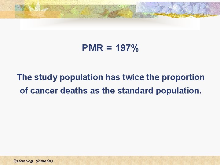
PMR = 197% The study population has twice the proportion of cancer deaths as the standard population. Epidemiology (Schneider)

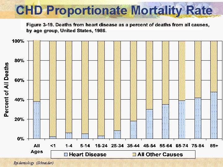
CHD Proportionate Mortality Rate Epidemiology (Schneider)

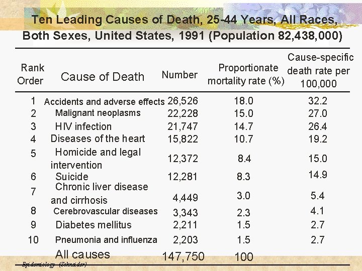
Ten Leading Causes of Death, 25 -44 Years, All Races, Both Sexes, United States, 1991 (Population 82, 438, 000) Rank Order Cause of Death Number 1 Accidents and adverse effects 26, 526 Malignant neoplasms 2 22, 228 3 HIV infection 21, 747 4 Diseases of the heart 15, 822 Homicide and legal 5 12, 372 intervention 6 Suicide 12, 281 Chronic liver disease 7 4, 449 and cirrhosis 8 Cerebrovascular diseases 3, 343 9 Diabetes mellitus 2, 211 Pneumonia and influenza 10 2, 203 All causes Epidemiology (Schneider) 147, 750 Cause-specific Proportionate death rate per mortality rate (%) 100, 000 18. 0 15. 0 14. 7 10. 7 32. 2 27. 0 26. 4 19. 2 8. 4 15. 0 8. 3 14. 9 3. 0 5. 4 4. 1 2. 7 2. 3 1. 5 100

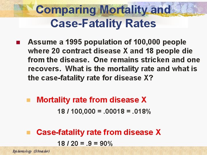
Comparing Mortality and Case-Fatality Rates n Assume a 1995 population of 100, 000 people where 20 contract disease X and 18 people die from the disease. One remains stricken and one recovers. What is the mortality rate and what is the case-fatality rate for disease X? n Mortality rate from disease X 18 / 100, 000 =. 00018 =. 018% n Case-fatality rate from disease X 18 / 20 =. 9 = 90% Epidemiology (Schneider)

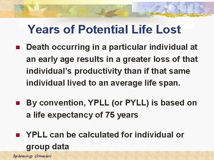
Years of Potential Life Lost n Death occurring in a particular individual at an early age results in a greater loss of that individual’s productivity than if that same individual lived to an average life span. n By convention, YPLL (or PYLL) is based on a life expectancy of 75 years n YPLL can be calculated for individual or group data Epidemiology (Schneider)

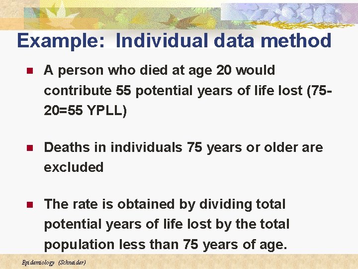
Example: Individual data method n A person who died at age 20 would contribute 55 potential years of life lost (7520=55 YPLL) n Deaths in individuals 75 years or older are excluded n The rate is obtained by dividing total potential years of life lost by the total population less than 75 years of age. Epidemiology (Schneider)

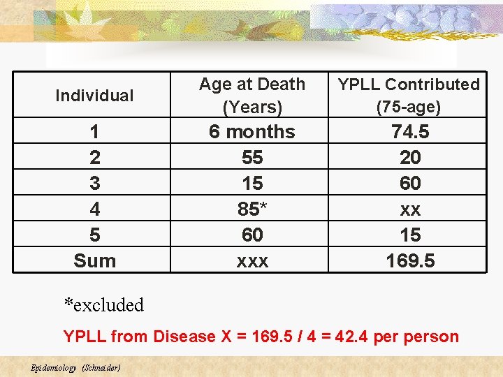
Individual Age at Death (Years) YPLL Contributed (75 -age) 1 2 3 4 5 Sum 6 months 55 15 85* 60 xxx 74. 5 20 60 xx 15 169. 5 *excluded YPLL from Disease X = 169. 5 / 4 = 42. 4 person Epidemiology (Schneider)

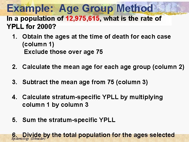
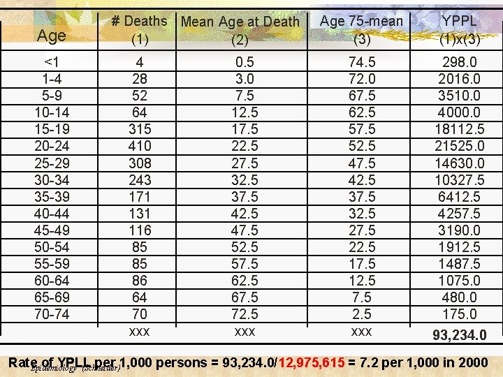
Example: Age Group Method In a population of 12, 975, 615, what is the rate of YPLL for 2000? 1. Obtain the ages at the time of death for each case (column 1) Exclude those over age 75 2. Calculate the mean age for each age group (column 2) 3. Subtract the mean age from 75 (column 3) 4. Calculate stratum-specific YPLL by multiplying column 1 by column 3 5. Sum the stratum-specific YPLL 6. Divide by the total population for the ages selected Epidemiology (Schneider)

Age <1 1 -4 5 -9 10 -14 15 -19 20 -24 25 -29 30 -34 35 -39 40 -44 45 -49 50 -54 55 -59 60 -64 65 -69 70 -74 # Deaths Mean Age at Death (1) (2) 4 28 52 64 315 410 308 243 171 131 116 85 85 86 64 70 xxx 0. 5 3. 0 7. 5 12. 5 17. 5 22. 5 27. 5 32. 5 37. 5 42. 5 47. 5 52. 5 57. 5 62. 5 67. 5 72. 5 xxx Age 75 -mean (3) YPPL (1)x(3) 74. 5 72. 0 67. 5 62. 5 57. 5 52. 5 47. 5 42. 5 37. 5 32. 5 27. 5 22. 5 17. 5 12. 5 7. 5 2. 5 xxx 298. 0 2016. 0 3510. 0 4000. 0 18112. 5 21525. 0 14630. 0 10327. 5 6412. 5 4257. 5 3190. 0 1912. 5 1487. 5 1075. 0 480. 0 175. 0 93, 234. 0 Rate. Epidemiology of YPLL per 1, 000 persons = 93, 234. 0/12, 975, 615 = 7. 2 per 1, 000 in 2000 (Schneider)

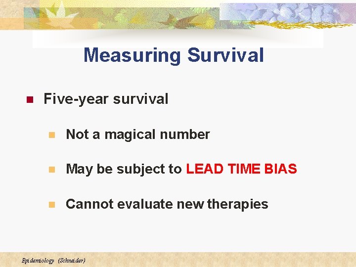
Measuring Survival n Five-year survival n Not a magical number n May be subject to LEAD TIME BIAS n Cannot evaluate new therapies Epidemiology (Schneider)

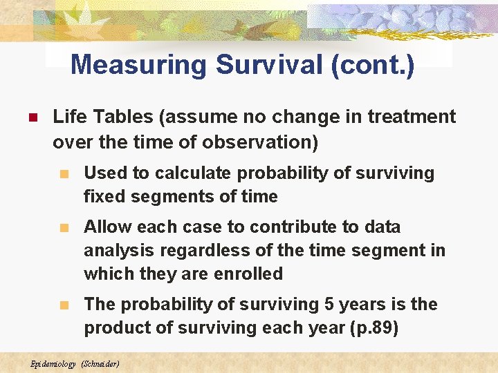
Measuring Survival (cont. ) n Life Tables (assume no change in treatment over the time of observation) n Used to calculate probability of surviving fixed segments of time n Allow each case to contribute to data analysis regardless of the time segment in which they are enrolled n The probability of surviving 5 years is the product of surviving each year (p. 89) Epidemiology (Schneider)

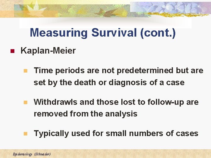
Measuring Survival (cont. ) n Kaplan-Meier n Time periods are not predetermined but are set by the death or diagnosis of a case n Withdrawls and those lost to follow-up are removed from the analysis n Typically used for small numbers of cases Epidemiology (Schneider)

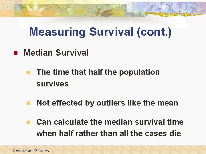
Measuring Survival (cont. ) n Median Survival n The time that half the population survives n Not effected by outliers like the mean n Can calculate the median survival time when half rather than all the cases die Epidemiology (Schneider)

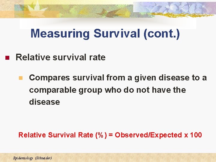
Measuring Survival (cont. ) n Relative survival rate n Compares survival from a given disease to a comparable group who do not have the disease Relative Survival Rate (%) = Observed/Expected x 100 Epidemiology (Schneider)