Smoothing This black art is why NLP is
Smoothing This black art is why NLP is taught in the engineering school. 600. 465 - Intro to NLP - J. Eisner 1

Parameter Estimation p(x 1=h, x 2=o, x 3=r, x 4=s, x 5=e, x 6=s, …) p(h | BOS, BOS) trigram model’s 4470/ 52108 parameters * p(o | BOS, h) 395/ 4470 * p(r | h, o) values of 1417/ 14765 those * p(s | o, r) 1573/ 26412 parameters, as naively * p(e | r, s) 1610/ 12253 estimated from Brown * p(s | s, e) 2044/ 21250 corpus. *… 600. 465 - Intro to NLP - J. Eisner 2
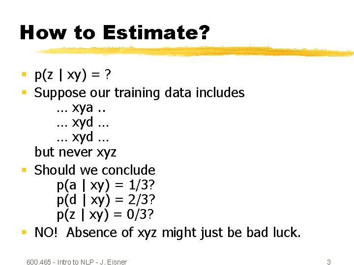
How to Estimate? § p(z | xy) = ? § Suppose our training data includes … xya. . … xyd … but never xyz § Should we conclude p(a | xy) = 1/3? p(d | xy) = 2/3? p(z | xy) = 0/3? § NO! Absence of xyz might just be bad luck. 600. 465 - Intro to NLP - J. Eisner 3
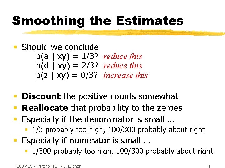
Smoothing the Estimates § Should we conclude p(a | xy) = 1/3? reduce this p(d | xy) = 2/3? reduce this p(z | xy) = 0/3? increase this § Discount the positive counts somewhat § Reallocate that probability to the zeroes § Especially if the denominator is small … § 1/3 probably too high, 100/300 probably about right § Especially if numerator is small … § 1/300 probably too high, 100/300 probably about right 600. 465 - Intro to NLP - J. Eisner 4
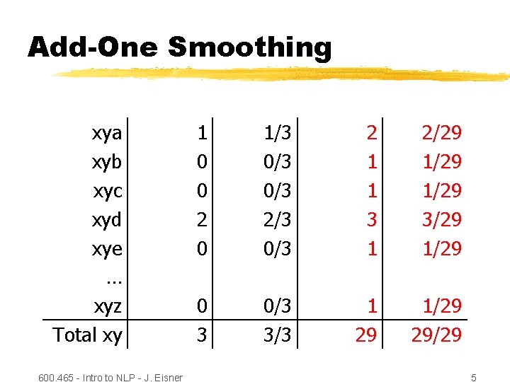
Add-One Smoothing xya xyb xyc xyd xye … xyz Total xy 600. 465 - Intro to NLP - J. Eisner 1 0 0 2 0 1/3 0/3 2/3 0/3 2 1 1 3 1 2/29 1/29 3/29 1/29 0 3 0/3 3/3 1 29 1/29 29/29 5
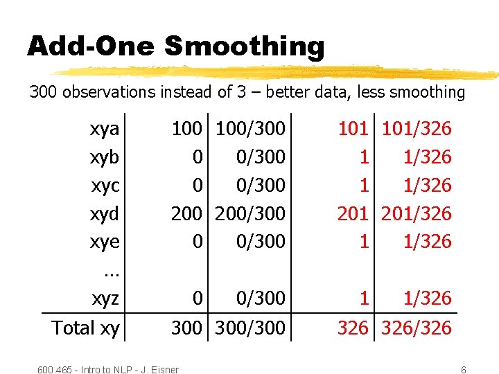
Add-One Smoothing 300 observations instead of 3 – better data, less smoothing xya xyb xyc xyd xye … xyz 100/300 0 0/300 200/300 0 0/300 Total xy 300/300 0 600. 465 - Intro to NLP - J. Eisner 0/300 101/326 1 1/326 201/326 1 1/326 326/326 6
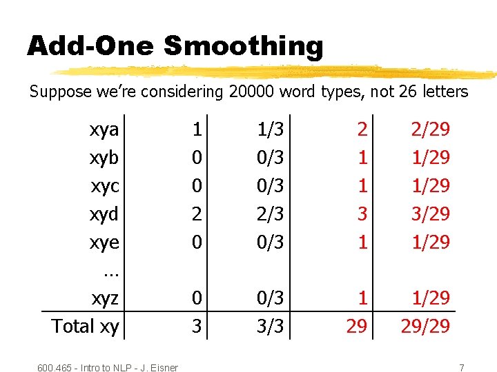
Add-One Smoothing Suppose we’re considering 20000 word types, not 26 letters xya xyb xyc xyd xye … xyz Total xy 600. 465 - Intro to NLP - J. Eisner 1 0 0 2 0 1/3 0/3 2/3 0/3 2 1 1 3 1 2/29 1/29 3/29 1/29 0 3 0/3 3/3 1 29 1/29 29/29 7
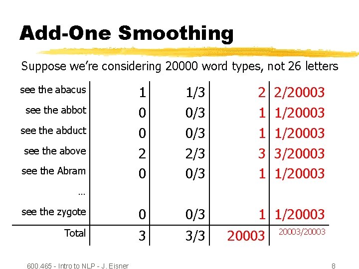
Add-One Smoothing Suppose we’re considering 20000 word types, not 26 letters 1 0 0 2 0 1/3 0/3 2/3 0/3 2 1 1 3 1 see the zygote 0 0/3 1 1/20003 Total 3 3/3 see the abacus see the abbot see the abduct see the above see the Abram 2/20003 1/20003 3/20003 1/20003 … 600. 465 - Intro to NLP - J. Eisner 20003/20003 8
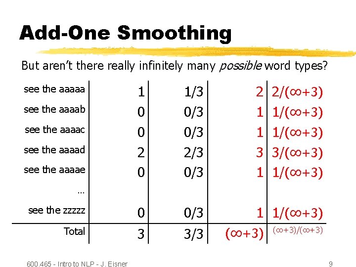
Add-One Smoothing But aren’t there really infinitely many possible word types? 1 0 0 2 0 1/3 0/3 2/3 0/3 2 1 1 3 1 see the zzzzz 0 0/3 1 1/(∞+3) Total 3 3/3 see the aaaaa see the aaaab see the aaaac see the aaaad see the aaaae 2/(∞+3) 1/(∞+3) 3/(∞+3) 1/(∞+3) … 600. 465 - Intro to NLP - J. Eisner (∞+3)/(∞+3) 9
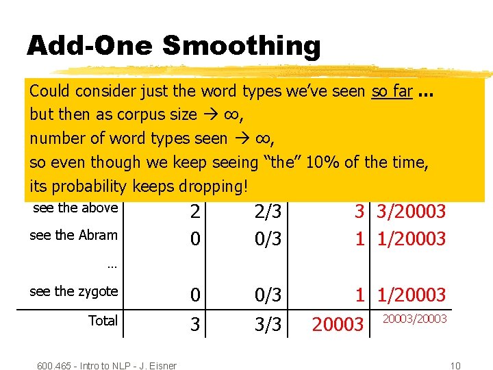
Add-One Smoothing Could consider just the word types we’ve seen so far … but then as corpus size ∞, see the abacus 1 1/3 2 2/20003 number of word types seen ∞, see the abbot 0 seeing 0/3 1/20003 so even though we keep “the” 10% of 1 the time, see the abduct 0 0/3 1 1/20003 its probability keeps dropping! 2 0 2/3 0/3 3 3/20003 1 1/20003 see the zygote 0 0/3 1 1/20003 Total 3 3/3 see the above see the Abram … 600. 465 - Intro to NLP - J. Eisner 20003/20003 10
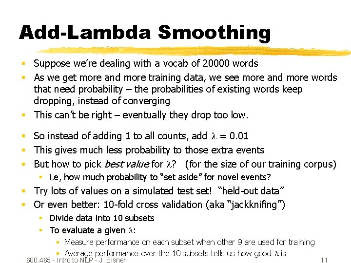
Add-Lambda Smoothing § Suppose we’re dealing with a vocab of 20000 words § As we get more and more training data, we see more and more words that need probability – the probabilities of existing words keep dropping, instead of converging § This can’t be right – eventually they drop too low. § So instead of adding 1 to all counts, add = 0. 01 § This gives much less probability to those extra events § But how to pick best value for ? (for the size of our training corpus) § i. e, how much probability to “set aside” for novel events? § Try lots of values on a simulated test set! “held-out data” § Or even better: 10 -fold cross validation (aka “jackknifing”) § Divide data into 10 subsets § To evaluate a given : § Measure performance on each subset when other 9 are used for training § Average performance over the 10 subsets tells us how good is 600. 465 - Intro to NLP - J. Eisner 11
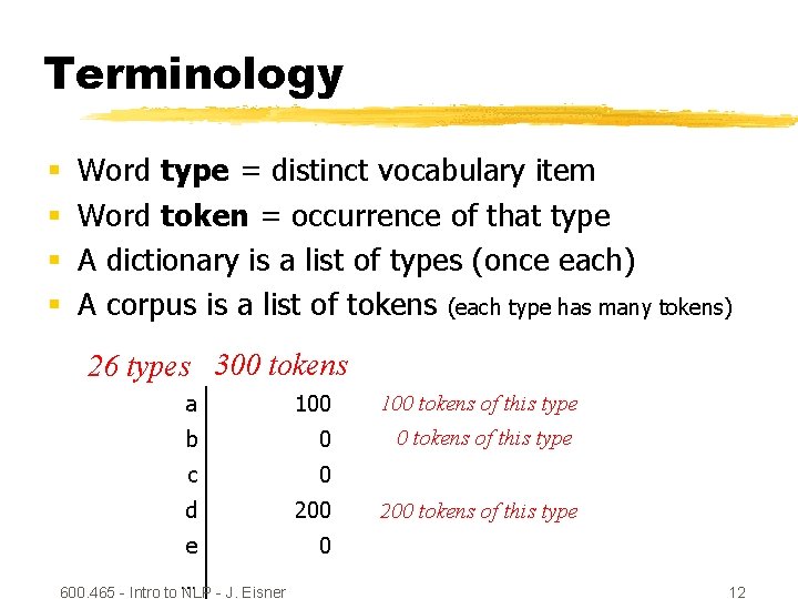
Terminology § § Word type = distinct vocabulary item Word token = occurrence of that type A dictionary is a list of types (once each) A corpus is a list of tokens (each type has many tokens) 26 types 300 tokens a 100 tokens of this type b 0 0 tokens of this type c 0 d 200 e 0 … 600. 465 - Intro to NLP - J. Eisner 200 tokens of this type 12
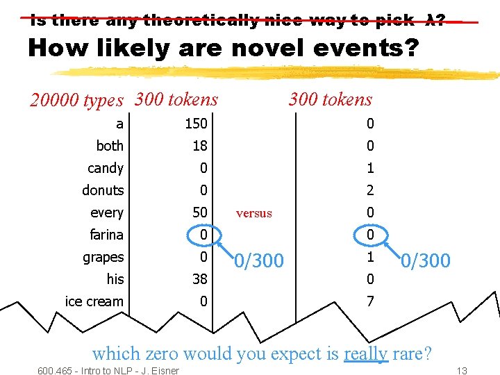
Is there any theoretically nice way to pick λ? How likely are novel events? 20000 types 300 tokens a 150 0 both 18 0 candy 0 1 donuts 0 2 every 50 farina 0 grapes 0 his 38 ice cream 0 versus 0 0 0/300 1 0 0/300 7 … which zero would you expect is really rare? 600. 465 - Intro to NLP - J. Eisner 13
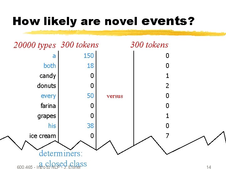
How likely are novel events? 20000 types 300 tokens a 150 0 both 18 0 candy 0 1 donuts 0 2 every 50 farina 0 0 grapes 0 1 his 38 0 ice cream 0 7 versus 0 … determiners: a closed class 600. 465 - Intro to NLP - J. Eisner 14
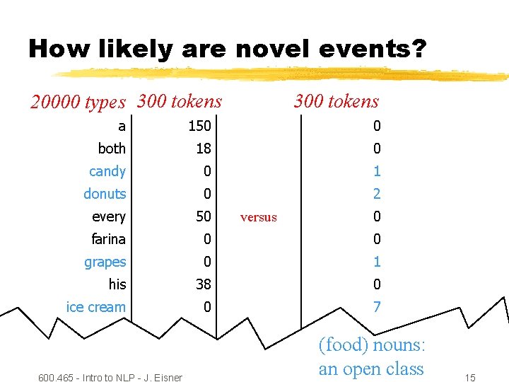
How likely are novel events? 20000 types 300 tokens a 150 0 both 18 0 candy 0 1 donuts 0 2 every 50 farina 0 0 grapes 0 1 his 38 0 ice cream 0 7 … 600. 465 - Intro to NLP - J. Eisner versus 0 (food) nouns: an open class 15
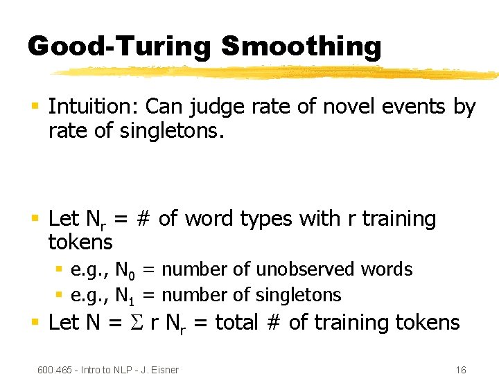
Good-Turing Smoothing § Intuition: Can judge rate of novel events by rate of singletons. § Let Nr = # of word types with r training tokens § e. g. , N 0 = number of unobserved words § e. g. , N 1 = number of singletons § Let N = r Nr = total # of training tokens 600. 465 - Intro to NLP - J. Eisner 16
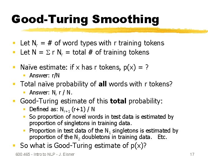
Good-Turing Smoothing § Let Nr = # of word types with r training tokens § Let N = r Nr = total # of training tokens § Naïve estimate: if x has r tokens, p(x) = ? § Answer: r/N § Total naïve probability of all words with r tokens? § Answer: Nr r / N. § Good-Turing estimate of this total probability: § Defined as: Nr+1 (r+1) / N § So proportion of novel words in test data is estimated by proportion of singletons in training data. § Proportion in test data of the N 1 singletons is estimated by proportion of the N 2 doubletons in training data. Etc. § So what is Good-Turing estimate of p(x)? 600. 465 - Intro to NLP - J. Eisner 17
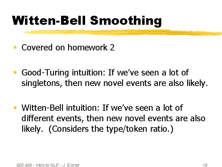
Witten-Bell Smoothing § Covered on homework 2 § Good-Turing intuition: If we’ve seen a lot of singletons, then new novel events are also likely. § Witten-Bell intuition: If we’ve seen a lot of different events, then new novel events are also likely. (Considers the type/token ratio. ) 600. 465 - Intro to NLP - J. Eisner 18
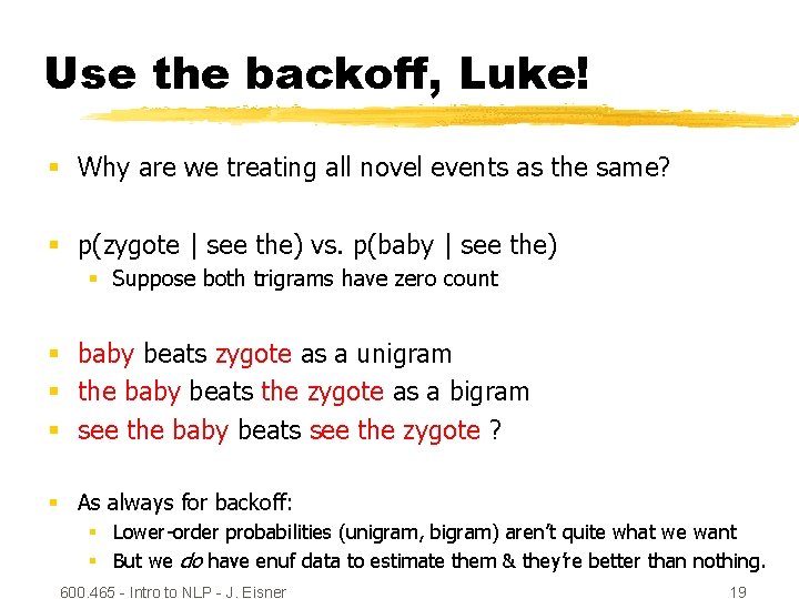
Use the backoff, Luke! § Why are we treating all novel events as the same? § p(zygote | see the) vs. p(baby | see the) § Suppose both trigrams have zero count § baby beats zygote as a unigram § the baby beats the zygote as a bigram § see the baby beats see the zygote ? § As always for backoff: § Lower-order probabilities (unigram, bigram) aren’t quite what we want § But we do have enuf data to estimate them & they’re better than nothing. 600. 465 - Intro to NLP - J. Eisner 19
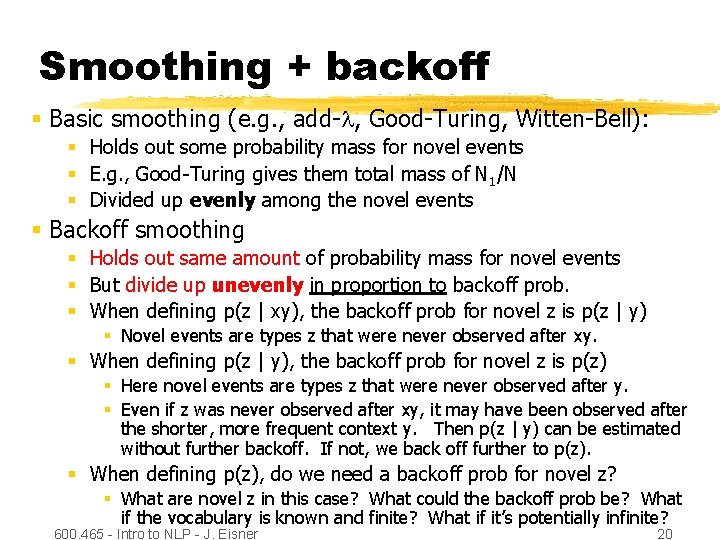
Smoothing + backoff § Basic smoothing (e. g. , add- , Good-Turing, Witten-Bell): § Holds out some probability mass for novel events § E. g. , Good-Turing gives them total mass of N 1/N § Divided up evenly among the novel events § Backoff smoothing § Holds out same amount of probability mass for novel events § But divide up unevenly in proportion to backoff prob. § When defining p(z | xy), the backoff prob for novel z is p(z | y) § Novel events are types z that were never observed after xy. § When defining p(z | y), the backoff prob for novel z is p(z) § Here novel events are types z that were never observed after y. § Even if z was never observed after xy, it may have been observed after the shorter, more frequent context y. Then p(z | y) can be estimated without further backoff. If not, we back off further to p(z). § When defining p(z), do we need a backoff prob for novel z? § What are novel z in this case? What could the backoff prob be? What if the vocabulary is known and finite? What if it’s potentially infinite? 600. 465 - Intro to NLP - J. Eisner 20
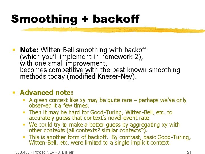
Smoothing + backoff § Note: Witten-Bell smoothing with backoff (which you’ll implement in homework 2), with one small improvement, becomes competitive with the best known smoothing methods today (modified Kneser-Ney). § Advanced note: § A given context like xy may be quite rare – perhaps we’ve only observed it a few times. § Then it may be hard for Good-Turing, Witten-Bell, etc. to accurately guess that context’s novel-event rate § We could try to make a better guess by aggregating xy with other contexts (all contexts? similar contexts? ). § This is another form of backoff. By contrast, basic Good-Turing, Witten-Bell, etc. were limited to a single implicit context. 600. 465 - Intro to NLP - J. Eisner 21
Deleted Interpolation § Can do even simpler stuff: § Estimate p(z | xy) as weighted average of the naïve MLE estimates of p(z | xy), p(z | y), p(z) § The weights can depend on the context xy § If a lot of data are available for the context, then trust p(z | xy) more since well-observed § If there are not many singletons in the context, then trust p(z | xy) more since closed-class § Learn the weights on held-out data w/ jackknifing § Different weights when xy is observed 1 time, 2 times, 3 -5 times, … 600. 465 - Intro to NLP - J. Eisner 22
- Slides: 22