Smith Chart Tutorial A D Snider August 2008

Smith Chart • Tutorial: A D Snider August 2008

Smith Chart • Tutorial: A D Snider August 2008 Impedance = Resistance + j*Reactance Admittance = Conductance + j*Susceptance

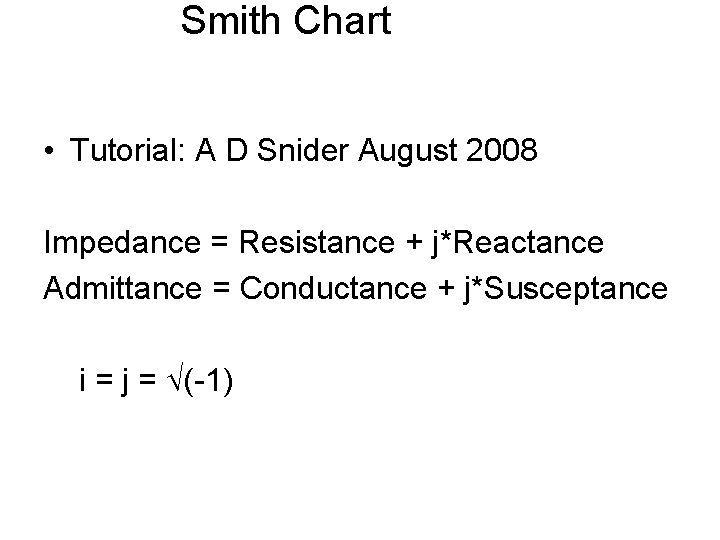
Smith Chart • Tutorial: A D Snider August 2008 Impedance = Resistance + j*Reactance Admittance = Conductance + j*Susceptance i = j = (-1)

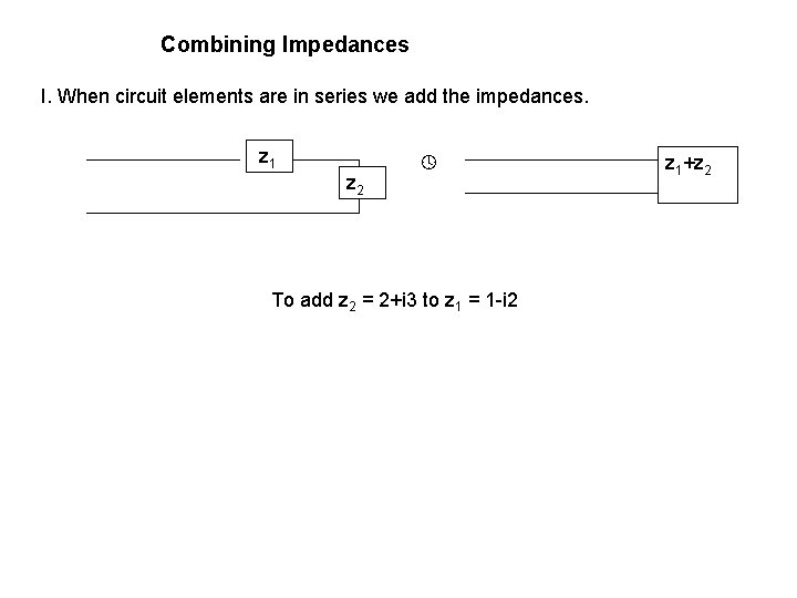
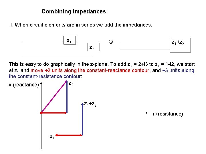
Combining Impedances I. When circuit elements are in series we add the impedances. z 1 z 2 To add z 2 = 2+i 3 to z 1 = 1 -i 2 z 1+z 2

Combining Impedances I. When circuit elements are in series we add the impedances. z 1 z 2 z 1+z 2 This is easy to do graphically in the z-plane. To add z 2 = 2+i 3 to z 1 = 1 -i 2, we start at z 1 and move +2 units along the constant-reactance contour, and +3 units along the constant-resistance contour: z 2 x (reactance) z 1+z 2 r (resistance) z 1

Combining Impedances II. When circuit elements are in parallel we add the admittances. z 1 z 2 z 1 z 2/(z 1+z 2) This is easy to do graphically in the y-plane; y=1/z. To add y 2 = 2+i 3 to y 1 = 1 -i 2,

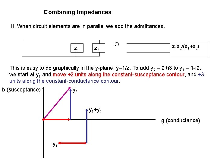
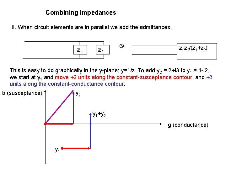
Combining Impedances II. When circuit elements are in parallel we add the admittances. z 1 z 2 z 1 z 2/(z 1+z 2) This is easy to do graphically in the y-plane; y=1/z. To add y 2 = 2+i 3 to y 1 = 1 -i 2, we start at y 1 and move +2 units along the constant-susceptance contour, and +3 units along the constant-conductance contour: b (susceptance) y 2 y 1+y 2 g (conductance) y 1

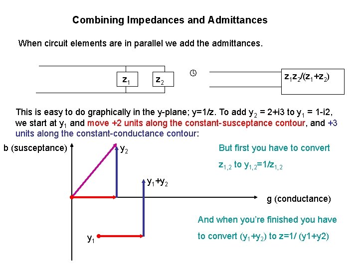
Combining Impedances and Admittances When circuit elements are in parallel we add the admittances. z 1 z 2 z 1 z 2/(z 1+z 2) This is easy to do graphically in the y-plane; y=1/z. To add y 2 = 2+i 3 to y 1 = 1 -i 2, we start at y 1 and move +2 units along the constant-susceptance contour, and +3 units along the constant-conductance contour: b (susceptance) y 2 But first you have to convert z 1, 2 to y 1, 2=1/z 1, 2 y 1+y 2 g (conductance) And when you’re finished you have y 1 to convert (y 1+y 2) to z=1/ (y 1+y 2)

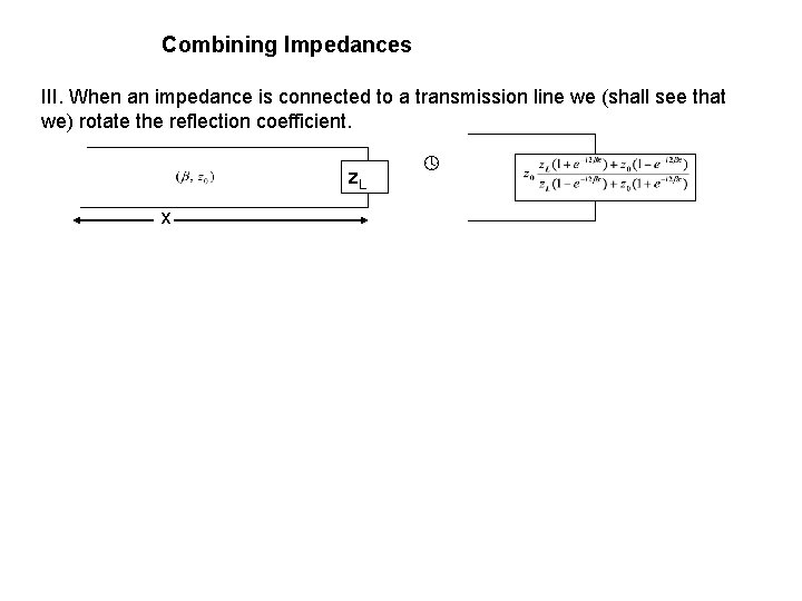
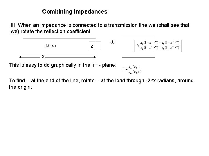
Combining Impedances III. When an impedance is connected to a transmission line we (shall see that we) rotate the reflection coefficient. z. L x

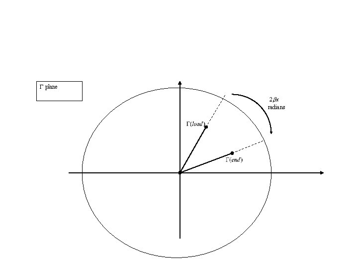
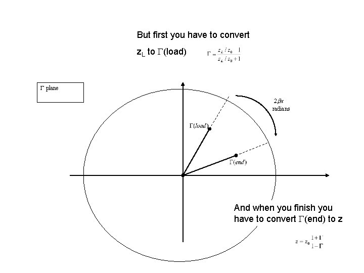
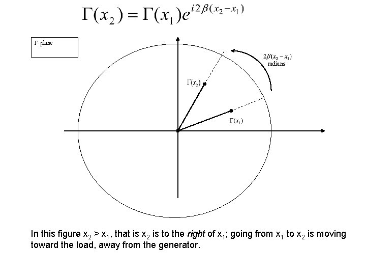
Combining Impedances III. When an impedance is connected to a transmission line we (shall see that we) rotate the reflection coefficient. z. L x This is easy to do graphically in the - plane; To find at the end of the line, rotate at the load through -2 x radians, around the origin:

plane radians

But first you have to convert z. L to (load) plane radians And when you finish you have to convert (end) to z

Digression • Transmission line theory

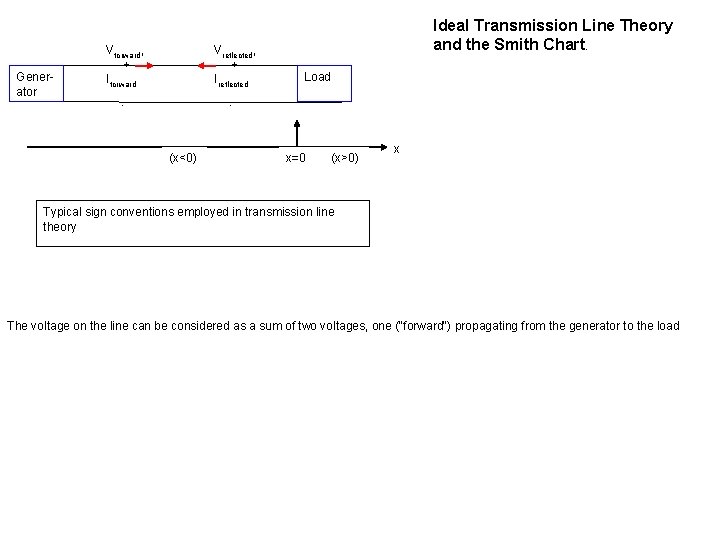
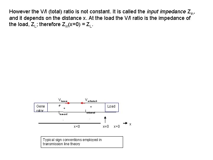
Generator Vforward, + Iforward Vreflected, + Ireflected - Ideal Transmission Line Theory and the Smith Chart. Load - (x<0) x=0 (x>0) x Typical sign conventions employed in transmission line theory The voltage on the line can be considered as a sum of two voltages, one ("forward") propagating from the generator to the load

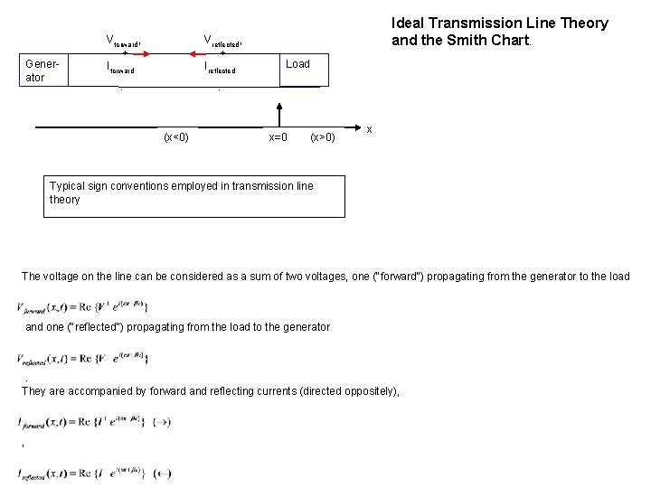
Generator Vforward, + Iforward Vreflected, + Ireflected - Ideal Transmission Line Theory and the Smith Chart. Load - (x<0) x=0 (x>0) x Typical sign conventions employed in transmission line theory The voltage on the line can be considered as a sum of two voltages, one ("forward") propagating from the generator to the load and one ("reflected") propagating from the load to the generator . They are accompanied by forward and reflecting currents (directed oppositely), ,

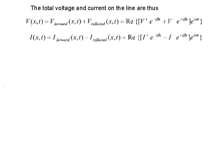
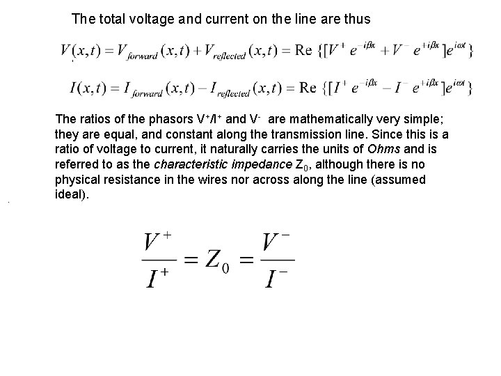
The total voltage and current on the line are thus , .

The total voltage and current on the line are thus , . The ratios of the phasors V+/I+ and V- are mathematically very simple; they are equal, and constant along the transmission line. Since this is a ratio of voltage to current, it naturally carries the units of Ohms and is referred to as the characteristic impedance Z 0, although there is no physical resistance in the wires nor across along the line (assumed ideal).

However the V/I (total) ratio is not constant. It is called the input impedance Zin, and it depends on the distance x. At the load the V/I ratio is the impedance of the load, ZL; therefore Zin(x=0) = ZL. Gene rator Vforwar d, + Iforward Vreflected, + Load Ireflected - - x<0 Typical sign conventions employed in transmission line theory x=0 x>0 x

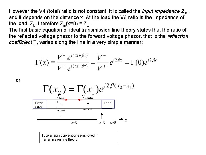
However the V/I (total) ratio is not constant. It is called the input impedance Zin, and it depends on the distance x. At the load the V/I ratio is the impedance of the load, ZL; therefore Zin(x=0) = ZL. The first basic equation of ideal transmission line theory states that the ratio of the reflected voltage phasor to the forward voltage phasor, that is the reflection coefficient , varies along the line in a very simple manner: or Gene rator Vforwar d, + Iforward Vreflected, + Load Ireflected - - x<0 Typical sign conventions employed in transmission line theory x=0 x>0 x

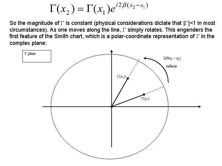
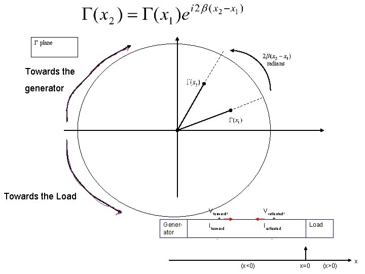
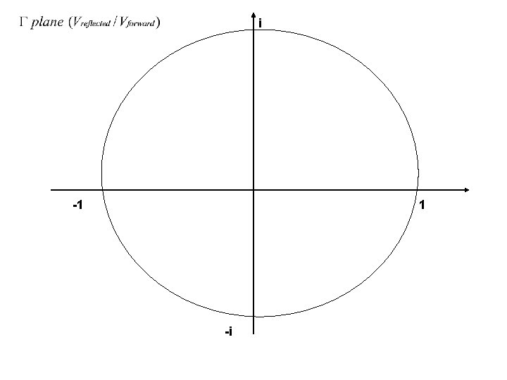
So the magnitude of is constant (physical considerations dictate that | |<1 in most circumstances). As one moves along the line, simply rotates. This engenders the first feature of the Smith chart, which is a polar-coordinate representation of in the complex plane: plane radians

plane radians In this figure x 2 > x 1, that is x 2 is to the right of x 1; going from x 1 to x 2 is moving toward the load, away from the generator.

plane radians Towards the generator Towards the Load Generator Vforward, + Iforward Vreflected, + Ireflected - Load - (x<0) x=0 (x>0) x

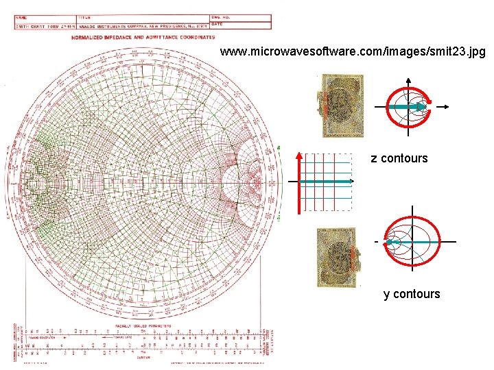
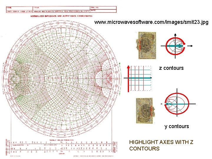
www. microwavesoftware. com/images/smit 23. jpg Here’s a full-blown Smith chart; the next 2 slides show closeups of the printing:

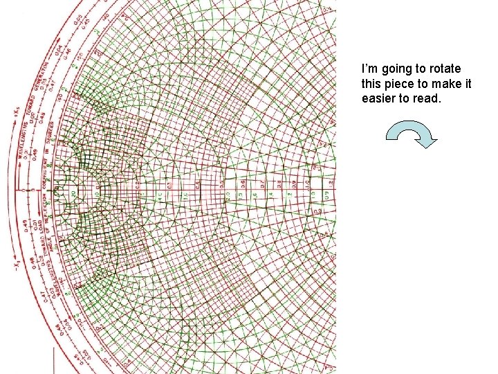
I’m going to rotate this piece to make it easier to read.

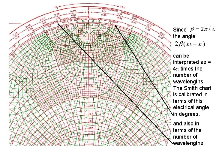
Since the angle can be interpreted as = 4 times the number of wavelengths. The Smith chart is calibrated in terms of this electrical angle in degrees, and also in terms of the number of wavelengths.

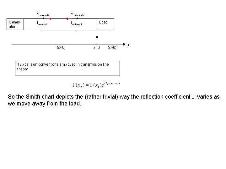
Generator Vforward, + Iforward Vreflected, + Ireflected - Load - (x<0) x=0 (x>0) x Typical sign conventions employed in transmission line theory So the Smith chart depicts the (rather trivial) way the reflection coefficient varies as we move away from the load.

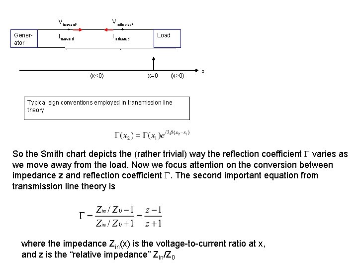
Generator Vforward, + Iforward Vreflected, + Ireflected - Load - (x<0) x=0 (x>0) x Typical sign conventions employed in transmission line theory So the Smith chart depicts the (rather trivial) way the reflection coefficient varies as we move away from the load. Now we focus attention on the conversion between impedance z and reflection coefficient . The second important equation from transmission line theory is where the impedance Zin(x) is the voltage-to-current ratio at x, and z is the “relative impedance” Zin/Z 0

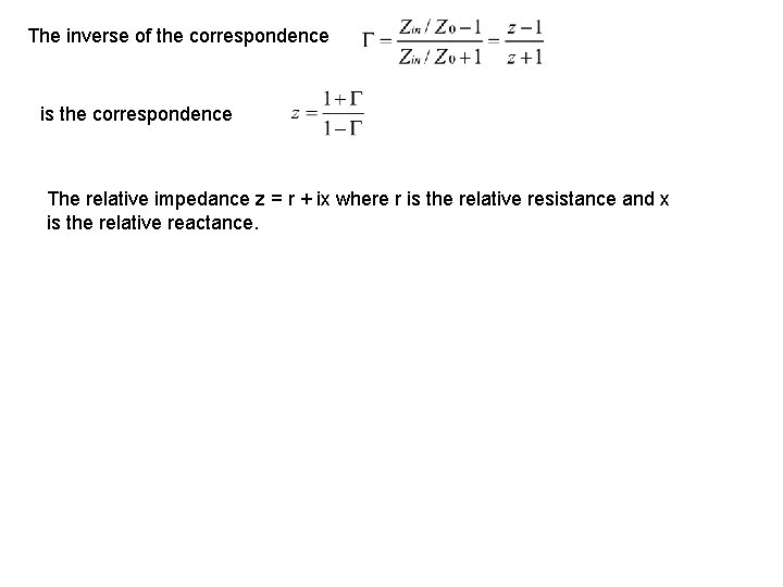
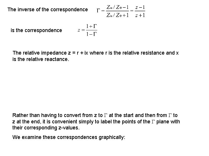
The inverse of the correspondence is the correspondence The relative impedance z = r + ix where r is the relative resistance and x is the relative reactance.

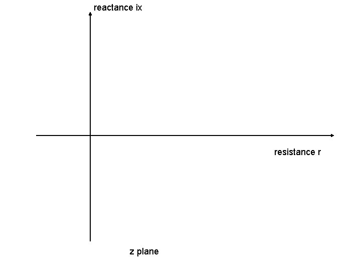
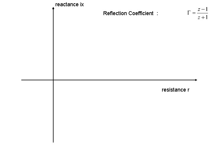
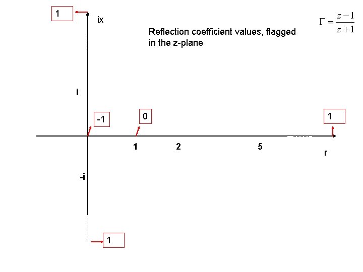
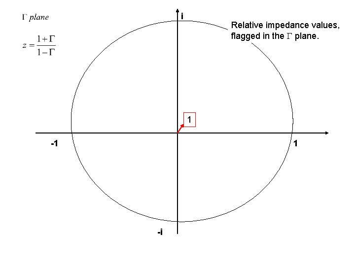
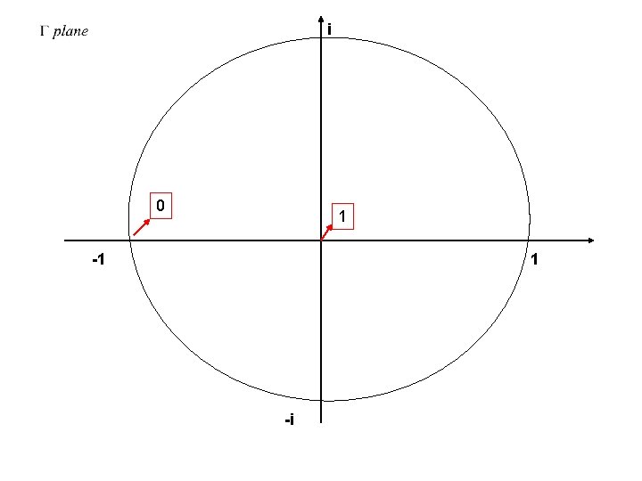
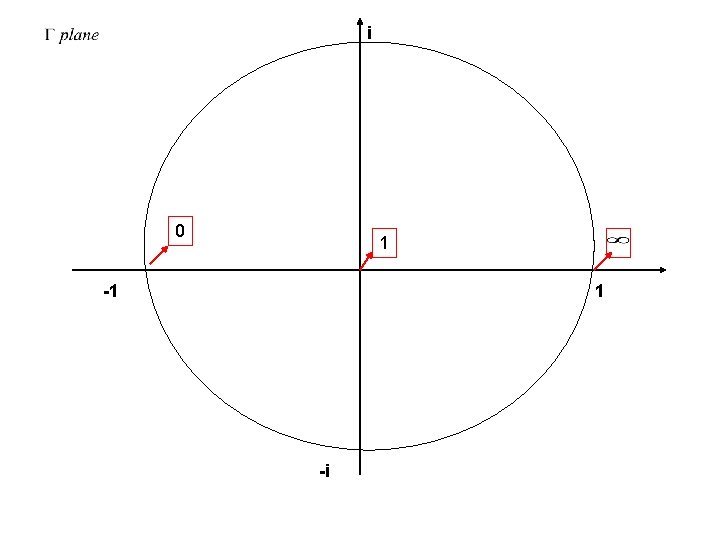
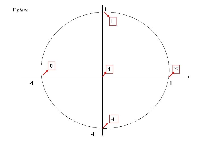
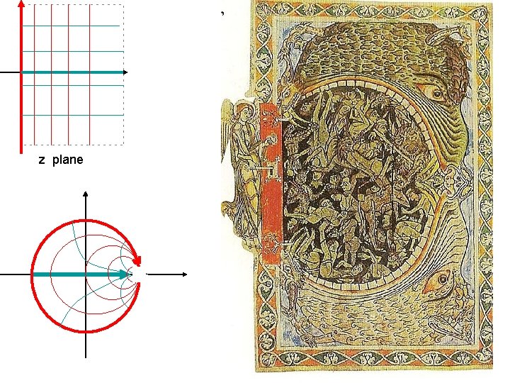
The inverse of the correspondence is the correspondence The relative impedance z = r + ix where r is the relative resistance and x is the relative reactance. Rather than having to convert from z to at the start and then from to z at the end, it is convenient simply to label the points of the plane with their corresponding z-values. We examine these correspondences graphically:

reactance ix resistance r z plane

reactance ix Reflection Coefficient : resistance r

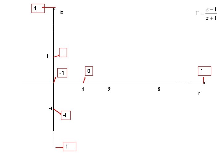
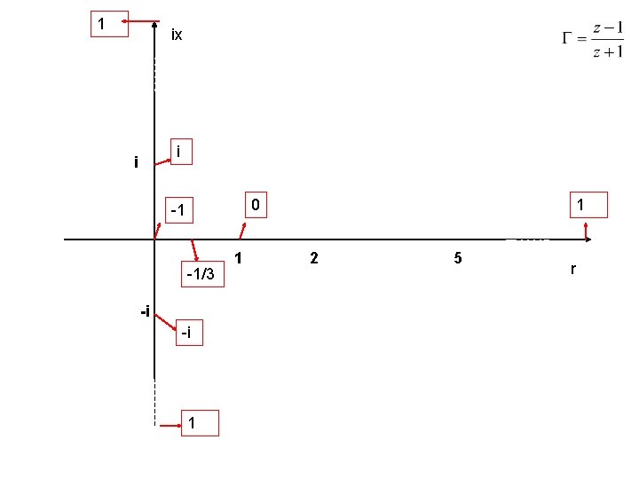
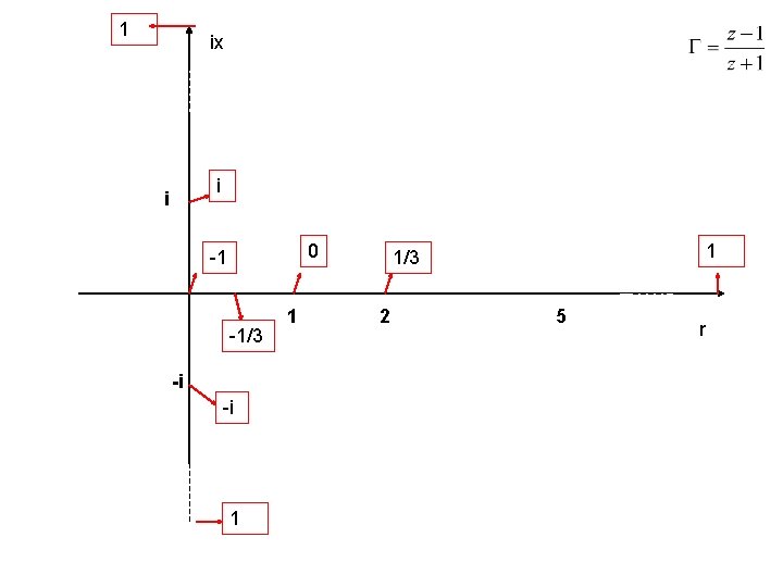
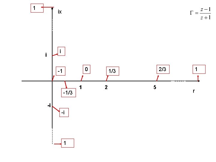
1 ix Reflection coefficient values, flagged in the z-plane i 0 -1 1 -i 1 1 2 5 r

1 ix i i 0 -1 1 -i -i 1 1 2 5 r

1 ix i i 0 -1 -1/3 -i -i 1 1 1 2 5 r

1 ix i i 0 -1 -1/3 -i -i 1 1/3 2 5 r

1 ix i i 0 -1 -1/3 -i -i 1 1 2/3 1/3 2 5 1 r

i -1 1 -i

i Relative impedance values, flagged in the plane. 1 -1 1 -i

i 0 1 -1 1 -i

i 0 1 -1 1 -i

i i 0 1 -1 1 -i -i

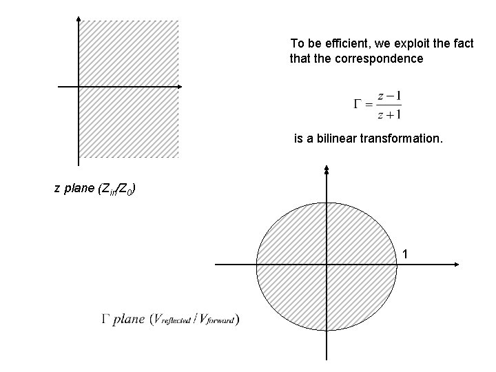
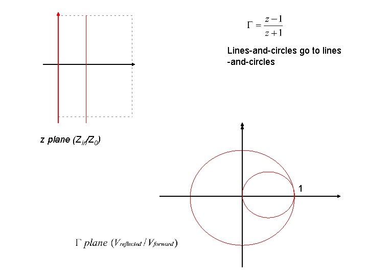
To be efficient, we exploit the fact that the correspondence is a bilinear transformation. z plane (Zin/Z 0) 1

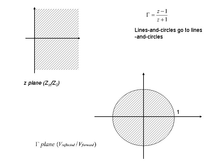
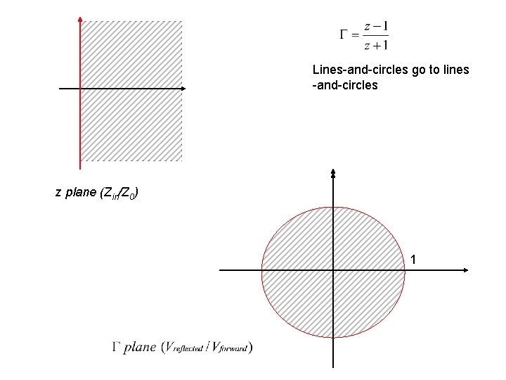
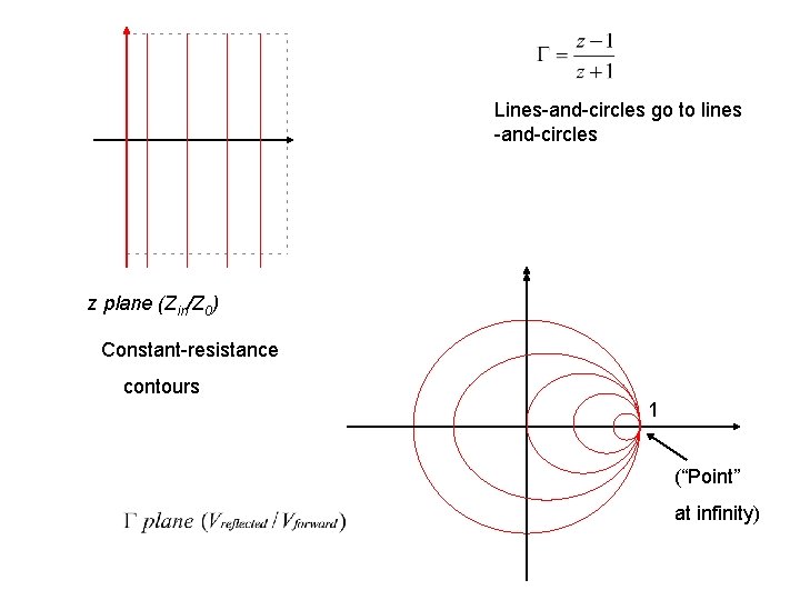
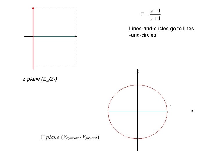
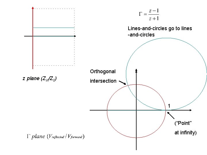
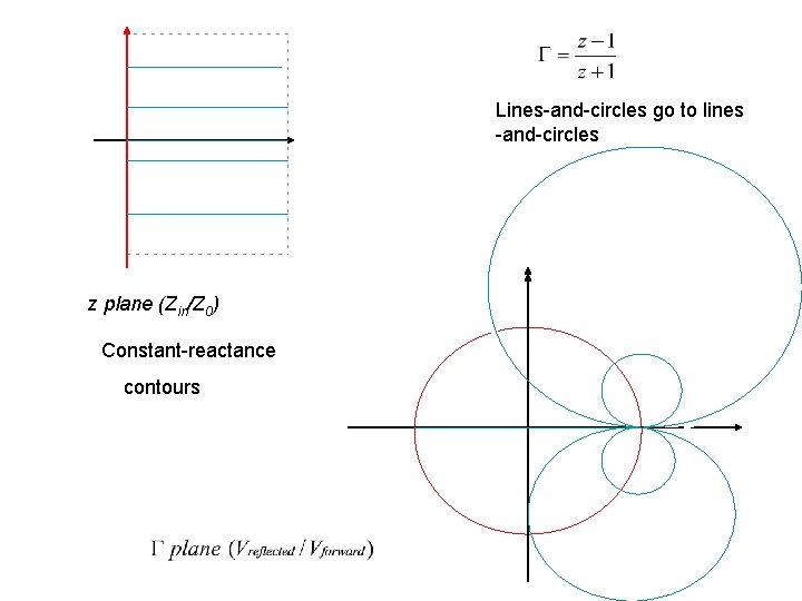
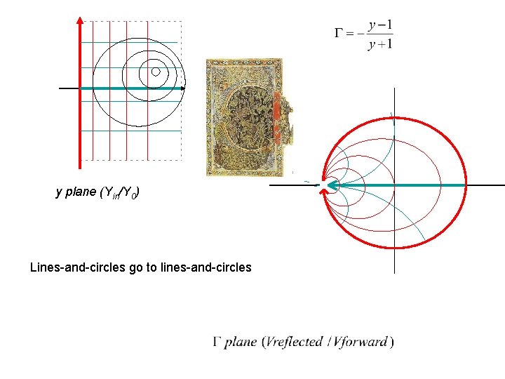
Lines-and-circles go to lines -and-circles z plane (Zin/Z 0) 1

Lines-and-circles go to lines -and-circles z plane (Zin/Z 0) 1

Lines-and-circles go to lines -and-circles z plane (Zin/Z 0) 1

Lines-and-circles go to lines -and-circles z plane (Zin/Z 0) Constant-resistance contours 1 (“Point” at infinity)

Lines-and-circles go to lines -and-circles z plane (Zin/Z 0) 1

Lines-and-circles go to lines -and-circles Orthogonal z plane (Zin/Z 0) intersection 1 (“Point” at infinity)

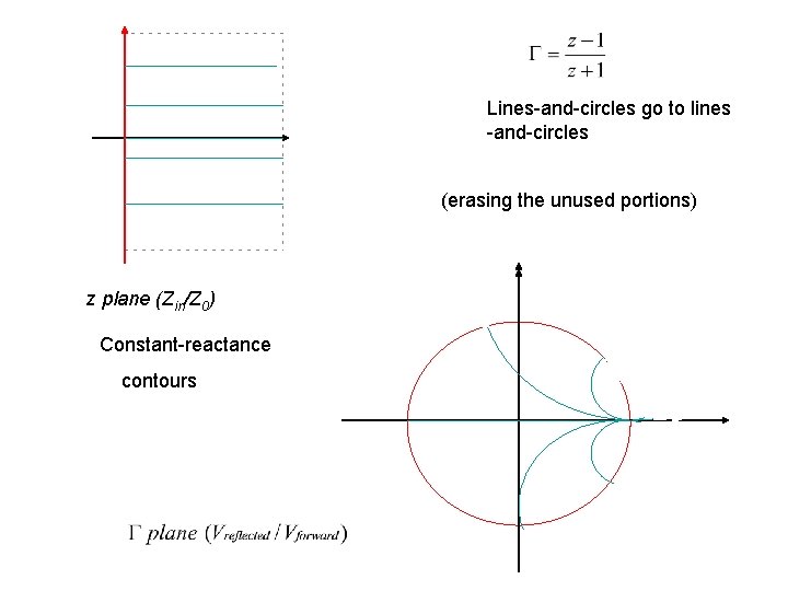
Lines-and-circles go to lines -and-circles z plane (Zin/Z 0) Constant-reactance contours

Lines-and-circles go to lines -and-circles (erasing the unused portions) z plane (Zin/Z 0) Constant-reactance contours

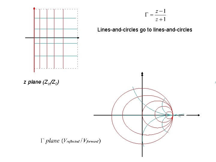
Lines-and-circles go to lines-and-circles z plane (Zin/Z 0)

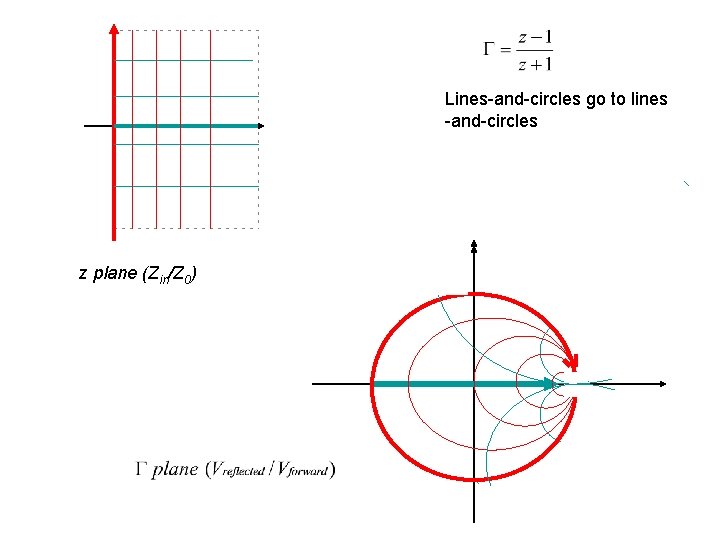
Lines-and-circles go to lines -and-circles z plane (Zin/Z 0)

z plane

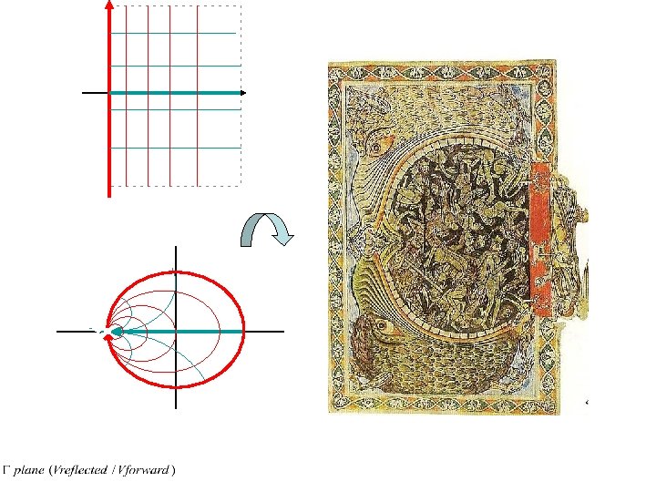
Ein Engel versperrt die Pforten der Unterwelt mit einem Schlüssel, Miniatur aus dem Psalter von Winchester, British Libary, London, 1150, artist unknown http: //en. wikipedia. org/wiki/Image: Ein_Engel_versperrt_die_Pforten_ der_Unterwelt_mit_einem_Schl% C 3%BCsel. jpg

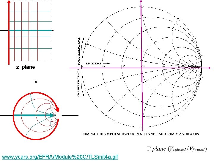
z plane www. ycars. org/EFRA/Module%20 C/TLSmit 4 a. gif

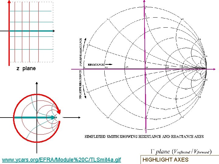
z plane www. ycars. org/EFRA/Module%20 C/TLSmit 4 a. gif HIGHLIGHT AXES

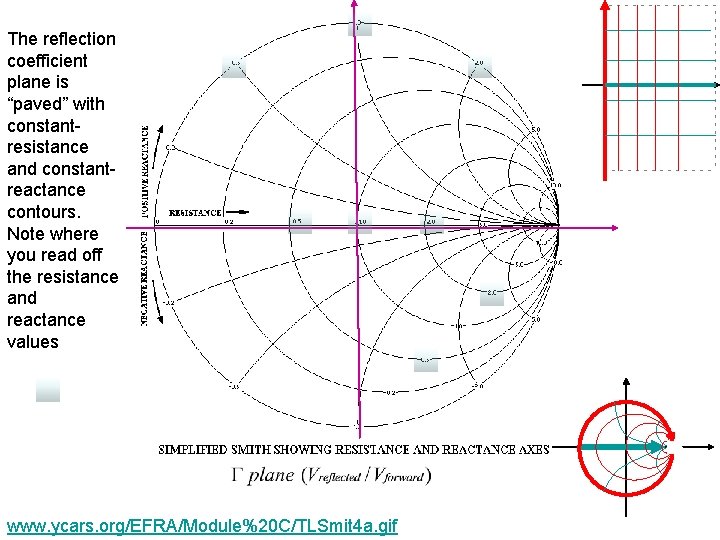
The reflection coefficient plane is “paved” with constantresistance and constantreactance contours. Note where you read off the resistance and reactance values www. ycars. org/EFRA/Module%20 C/TLSmit 4 a. gif

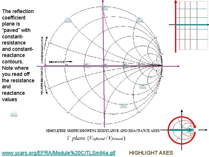
The reflection coefficient plane is “paved” with constantresistance and constantreactance contours. Note where you read off the resistance and reactance values www. ycars. org/EFRA/Module%20 C/TLSmit 4 a. gif HIGHLIGHT AXES

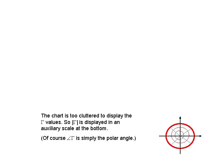
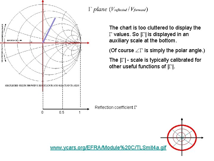
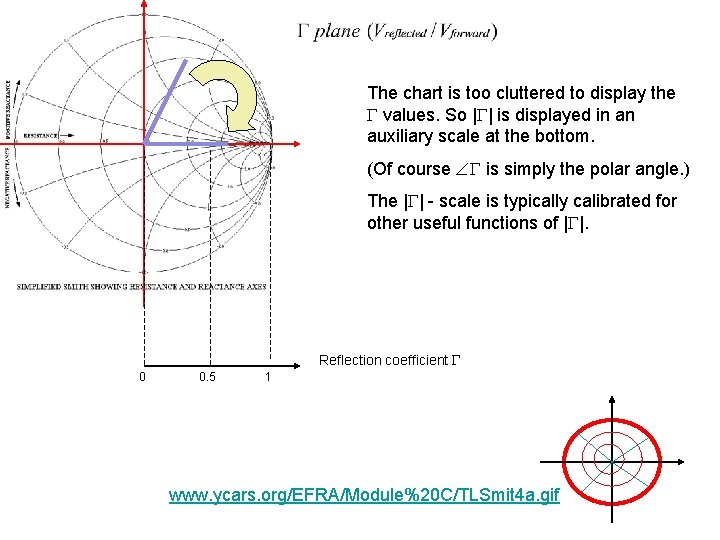
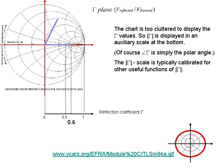
The chart is too cluttered to display the values. So | | is displayed in an auxiliary scale at the bottom. (Of course is simply the polar angle. )

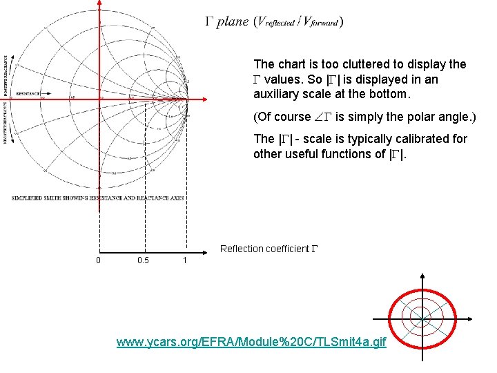
The chart is too cluttered to display the values. So | | is displayed in an auxiliary scale at the bottom. (Of course is simply the polar angle. ) The | | - scale is typically calibrated for other useful functions of | |. Reflection coefficient 0 0. 5 1 www. ycars. org/EFRA/Module%20 C/TLSmit 4 a. gif

The chart is too cluttered to display the values. So | | is displayed in an auxiliary scale at the bottom. (Of course is simply the polar angle. ) The | | - scale is typically calibrated for other useful functions of | |. Reflection coefficient 0 0. 5 1 www. ycars. org/EFRA/Module%20 C/TLSmit 4 a. gif

The chart is too cluttered to display the values. So | | is displayed in an auxiliary scale at the bottom. (Of course is simply the polar angle. ) The | | - scale is typically calibrated for other useful functions of | |. Reflection coefficient 0 0. 5 1 www. ycars. org/EFRA/Module%20 C/TLSmit 4 a. gif

The chart is too cluttered to display the values. So | | is displayed in an auxiliary scale at the bottom. (Of course is simply the polar angle. ) The | | - scale is typically calibrated for other useful functions of | |. Reflection coefficient 0 0. 5 0. 6 1 www. ycars. org/EFRA/Module%20 C/TLSmit 4 a. gif

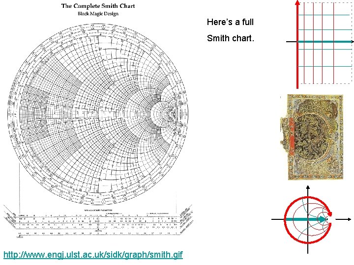
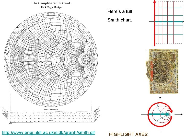
Here’s a full Smith chart. http: //www. engj. ulst. ac. uk/sidk/graph/smith. gif

Here’s a full Smith chart. http: //www. engj. ulst. ac. uk/sidk/graph/smith. gif HIGHLIGHT AXES

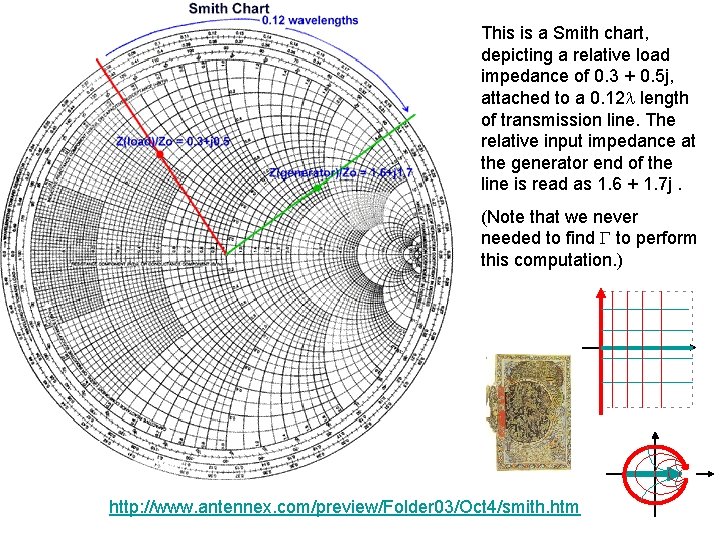
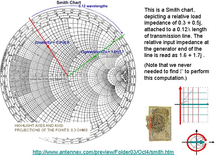
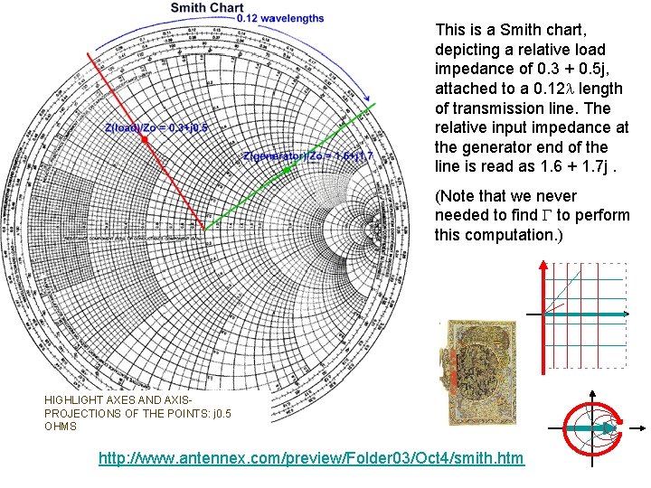
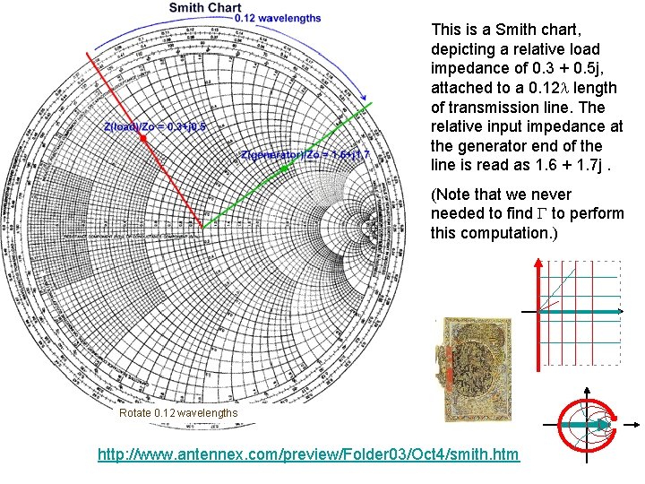
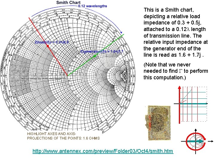
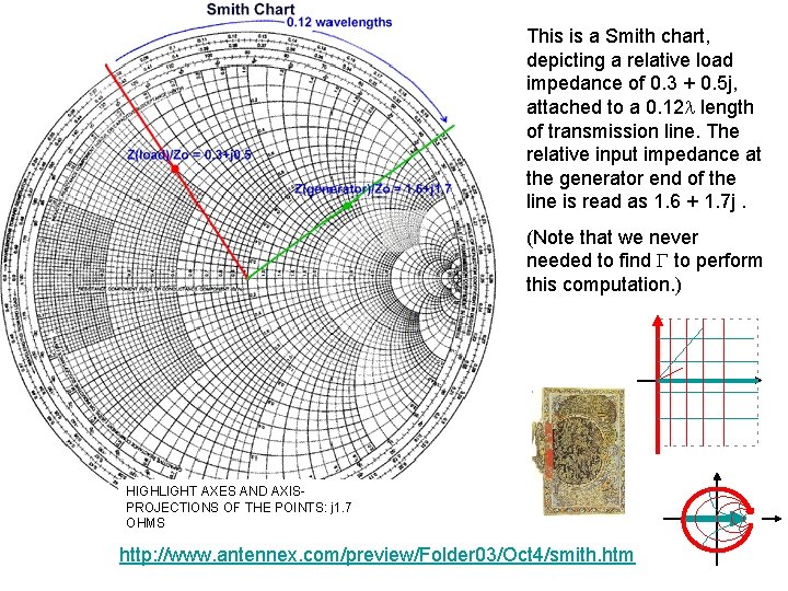
This is a Smith chart, depicting a relative load impedance of 0. 3 + 0. 5 j, attached to a 0. 12 length of transmission line. The relative input impedance at the generator end of the line is read as 1. 6 + 1. 7 j. (Note that we never needed to find to perform this computation. ) http: //www. antennex. com/preview/Folder 03/Oct 4/smith. htm

This is a Smith chart, depicting a relative load impedance of 0. 3 + 0. 5 j, attached to a 0. 12 length of transmission line. The relative input impedance at the generator end of the line is read as 1. 6 + 1. 7 j. (Note that we never needed to find to perform this computation. ) HIGHLIGHT AXES AND AXISPROJECTIONS OF THE POINTS: 0. 3 OHMS http: //www. antennex. com/preview/Folder 03/Oct 4/smith. htm

This is a Smith chart, depicting a relative load impedance of 0. 3 + 0. 5 j, attached to a 0. 12 length of transmission line. The relative input impedance at the generator end of the line is read as 1. 6 + 1. 7 j. (Note that we never needed to find to perform this computation. ) HIGHLIGHT AXES AND AXISPROJECTIONS OF THE POINTS: j 0. 5 OHMS http: //www. antennex. com/preview/Folder 03/Oct 4/smith. htm

This is a Smith chart, depicting a relative load impedance of 0. 3 + 0. 5 j, attached to a 0. 12 length of transmission line. The relative input impedance at the generator end of the line is read as 1. 6 + 1. 7 j. (Note that we never needed to find to perform this computation. ) Rotate 0. 12 wavelengths http: //www. antennex. com/preview/Folder 03/Oct 4/smith. htm

This is a Smith chart, depicting a relative load impedance of 0. 3 + 0. 5 j, attached to a 0. 12 length of transmission line. The relative input impedance at the generator end of the line is read as 1. 6 + 1. 7 j. (Note that we never needed to find to perform this computation. ) HIGHLIGHT AXES AND AXISPROJECTIONS OF THE POINTS: 1. 6 OHMS http: //www. antennex. com/preview/Folder 03/Oct 4/smith. htm

This is a Smith chart, depicting a relative load impedance of 0. 3 + 0. 5 j, attached to a 0. 12 length of transmission line. The relative input impedance at the generator end of the line is read as 1. 6 + 1. 7 j. (Note that we never needed to find to perform this computation. ) HIGHLIGHT AXES AND AXISPROJECTIONS OF THE POINTS: j 1. 7 OHMS http: //www. antennex. com/preview/Folder 03/Oct 4/smith. htm

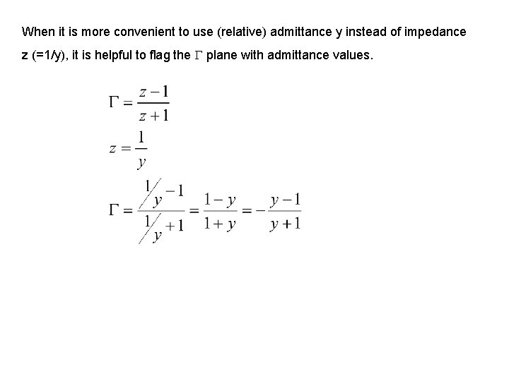
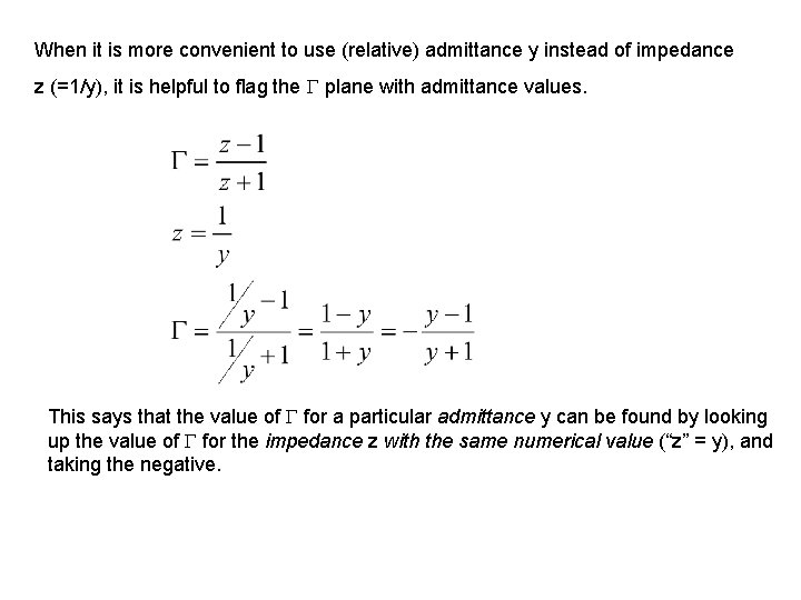
When it is more convenient to use (relative) admittance y instead of impedance z (=1/y), it is helpful to flag the plane with admittance values.

When it is more convenient to use (relative) admittance y instead of impedance z (=1/y), it is helpful to flag the plane with admittance values.

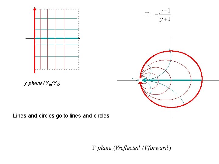
y plane (Yin/Y 0) Lines-and-circles go to lines-and-circles

When it is more convenient to use (relative) admittance y instead of impedance z (=1/y), it is helpful to flag the plane with admittance values. This says that the value of for a particular admittance y can be found by looking up the value of for the impedance z with the same numerical value (“z” = y), and taking the negative.

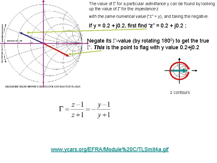
The value of for a particular admittance y can be found by looking up the value of for the impedance z with the same numerical value (“z” = y), and taking the negative. If y = 0. 2 + j 0. 2, first find “z” = 0. 2 + j 0. 2 ; Negate its -value (by rotating 1800) to get the true . This is the point to flag with y value 0. 2+j 0. 2 z contours www. ycars. org/EFRA/Module%20 C/TLSmit 4 a. gif

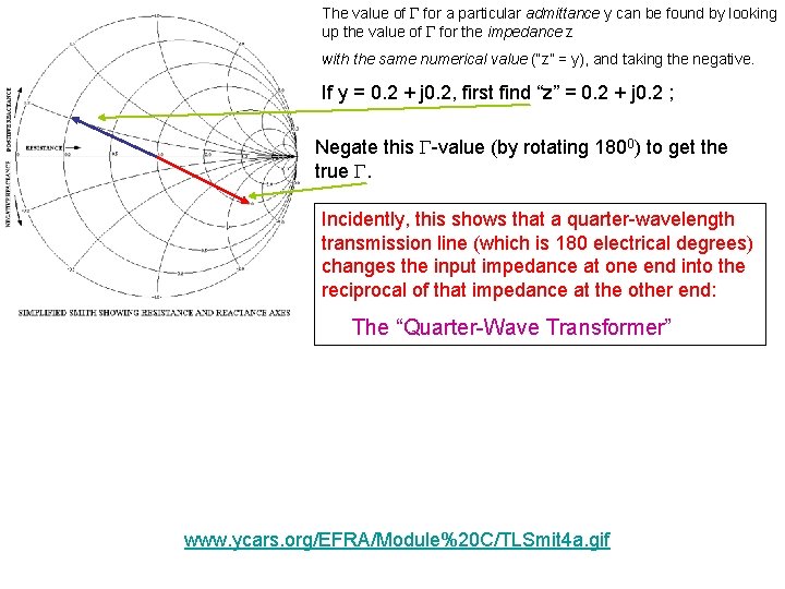
The value of for a particular admittance y can be found by looking up the value of for the impedance z with the same numerical value (“z” = y), and taking the negative. If y = 0. 2 + j 0. 2, first find “z” = 0. 2 + j 0. 2 ; Negate this -value (by rotating 1800) to get the true . Incidently, this shows that a quarter-wavelength transmission line (which is 180 electrical degrees) changes the input impedance at one end into the reciprocal of that impedance at the other end: The “Quarter-Wave Transformer” www. ycars. org/EFRA/Module%20 C/TLSmit 4 a. gif

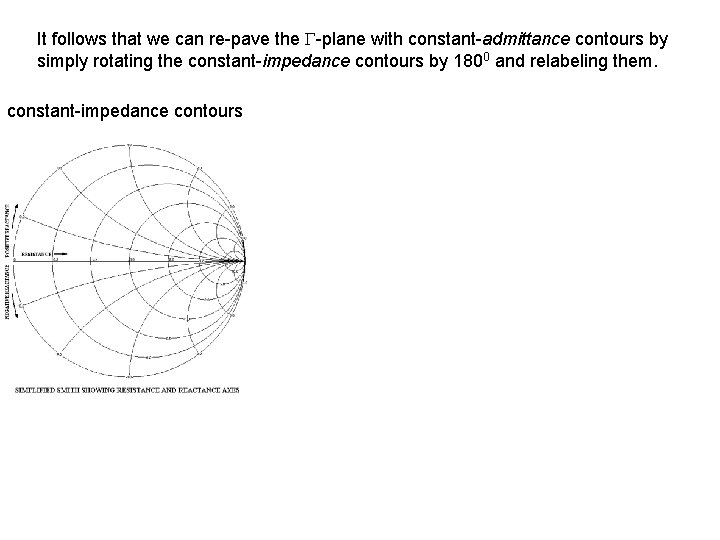
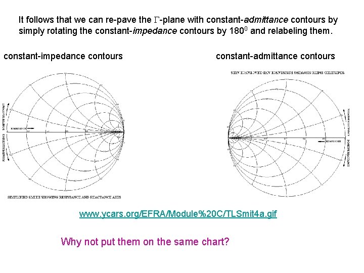
It follows that we can re-pave the -plane with constant-admittance contours by simply rotating the constant-impedance contours by 1800 and relabeling them.

It follows that we can re-pave the -plane with constant-admittance contours by simply rotating the constant-impedance contours by 1800 and relabeling them. constant-impedance contours

It follows that we can re-pave the -plane with constant-admittance contours by simply rotating the constant-impedance contours by 1800 and relabeling them. constant-impedance contours constant-admittance contours www. ycars. org/EFRA/Module%20 C/TLSmit 4 a. gif Why not put them on the same chart?

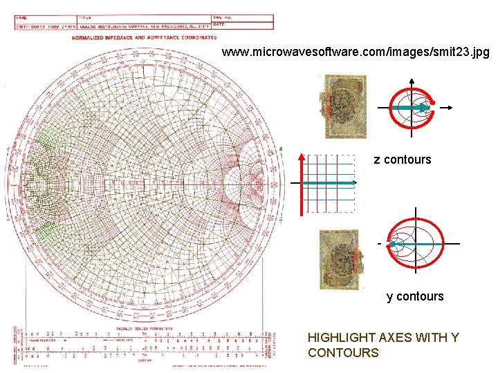
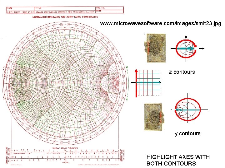
www. microwavesoftware. com/images/smit 23. jpg z contours y contours

www. microwavesoftware. com/images/smit 23. jpg z contours y contours HIGHLIGHT AXES WITH Z CONTOURS

www. microwavesoftware. com/images/smit 23. jpg z contours y contours HIGHLIGHT AXES WITH Y CONTOURS

www. microwavesoftware. com/images/smit 23. jpg z contours y contours HIGHLIGHT AXES WITH BOTH CONTOURS

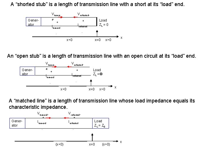
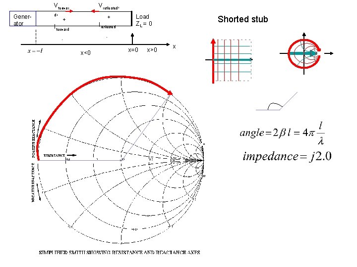
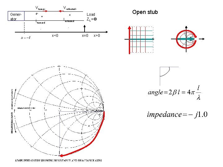
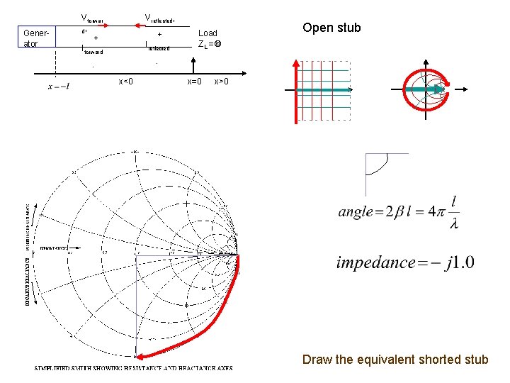
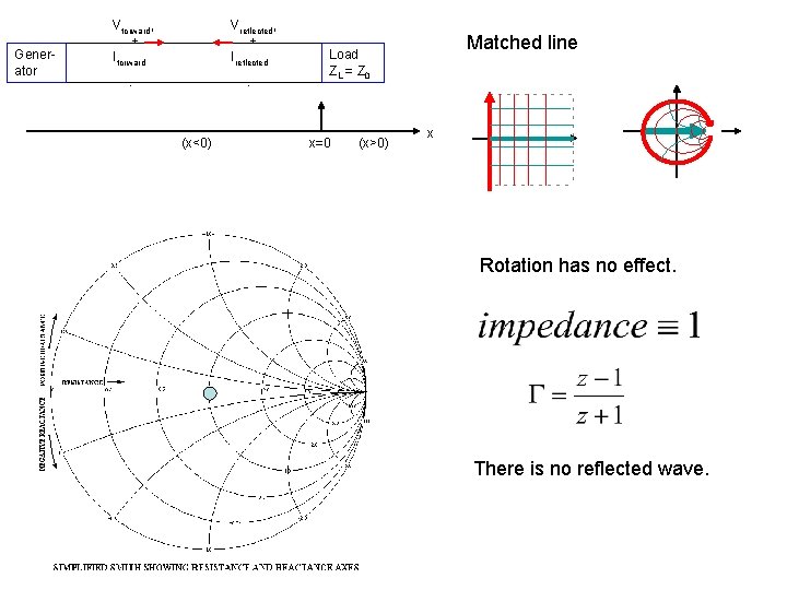
A “shorted stub” is a length of transmission line with a short at its “load” end. Vforwar d, + Iforward Generator Vreflected, Load ZL = 0 + Ireflected - - x<0 x=0 x x>0 An “open stub” is a length of transmission line with an open circuit at its “load” end. Vforwar d, + Iforward Generator Vreflected, + Ireflected Load ZL = - - x<0 x=0 x>0 x A “matched line” is a length of transmission line whose load impedance equals its characteristic impedance. Generator Vforward, + Iforward Vreflected, + Ireflected - - (x<0) Load ZL = Z 0 x=0 (x>0) x

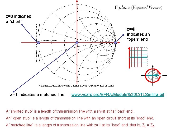
z=0 indicates a “short” z= indicates an “open” end z=1 indicates a matched line www. ycars. org/EFRA/Module%20 C/TLSmit 4 a. gif A “shorted stub” is a length of transmission line with a short at its “load” end. An “open stub” is a length of transmission line with an open circuit short at its “load” end. A “matched line” is a length of transmission line with z=1 at its “load” end; that is, Z L = Z 0.

Generator Vforwar d, + Iforward Vreflected, + Ireflected Load ZL = 0 Shorted stub - - x<0 x=0 x>0 x

Generator Vforwar d, + Iforward Vreflected, + Ireflected Load ZL = - - x<0 x=0 x>0 Open stub

Generator Vforwar d, + Iforward Vreflected, + Ireflected Load ZL = Open stub - - x<0 x=0 x>0 Draw the equivalent shorted stub

Generator Vforward, + Iforward Vreflected, + Ireflected - - (x<0) Matched line Load ZL = Z 0 x=0 (x>0) x Rotation has no effect. There is no reflected wave.

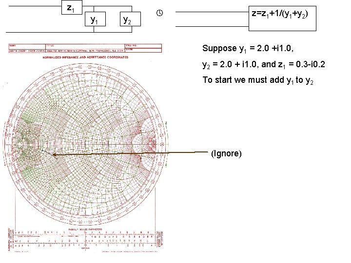
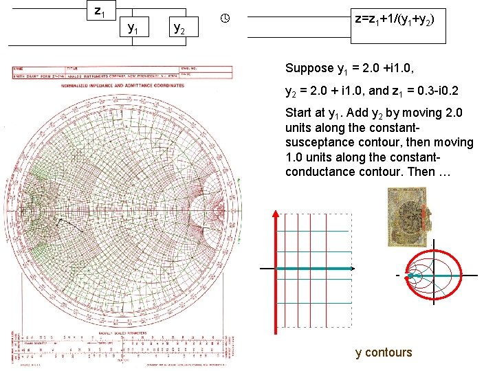
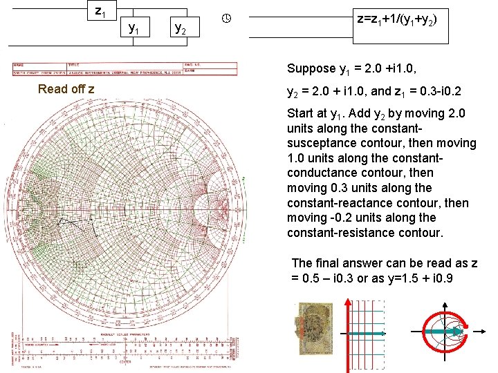
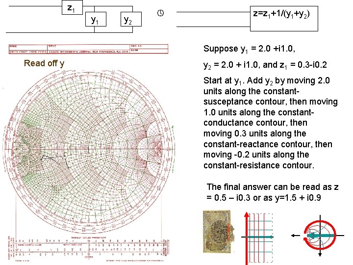
z 1 y 2 z=z 1+1/(y 1+y 2) Suppose y 1 = 2. 0 +i 1. 0, y 2 = 2. 0 + i 1. 0, and z 1 = 0. 3 -i 0. 2 To start we must add y 1 to y 2 (Ignore)

Combining Impedances II. When circuit elements are in parallel we add the admittances. z 1 z 2 z 1 z 2/(z 1+z 2) This is easy to do graphically in the y-plane; y=1/z. To add y 2 = 2+i 3 to y 1 = 1 -i 2, we start at y 1 and move +2 units along the constant-susceptance contour, and +3 units along the constant-conductance contour: b (susceptance) y 2 y 1+y 2 g (conductance) y 1

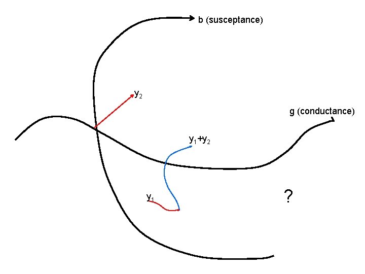
b (susceptance) y 2 g (conductance) y 1+y 2 y 1 ?

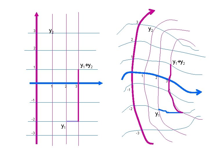
3 3 y 2 2 2 1 y 1+y 2 1 1 1 2 3 2 -1 -1 -2 y 1 -3 -3 3

z 1 y 2 z=z 1+1/(y 1+y 2) Suppose y 1 = 2. 0 +i 1. 0, y 2 = 2. 0 + i 1. 0, and z 1 = 0. 3 -i 0. 2 Start at y 1. Add y 2 by moving 2. 0 units along the constantsusceptance contour, then moving 1. 0 units along the constantconductance contour. Then … y contours

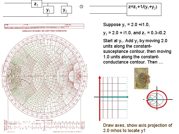
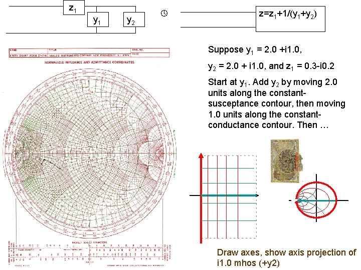
z 1 y 2 z=z 1+1/(y 1+y 2) Suppose y 1 = 2. 0 +i 1. 0, y 2 = 2. 0 + i 1. 0, and z 1 = 0. 3 -i 0. 2 Start at y 1. Add y 2 by moving 2. 0 units along the constantsusceptance contour, then moving 1. 0 units along the constantconductance contour. Then … Draw axes, show axis projection of y contours 2. 0 mhos to locate y 1

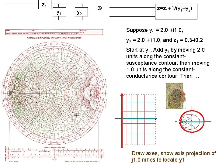
z 1 y 2 z=z 1+1/(y 1+y 2) Suppose y 1 = 2. 0 +i 1. 0, y 2 = 2. 0 + i 1. 0, and z 1 = 0. 3 -i 0. 2 Start at y 1. Add y 2 by moving 2. 0 units along the constantsusceptance contour, then moving 1. 0 units along the constantconductance contour. Then … Draw axes, y show axis projection of contours j 1. 0 mhos to locate y 1

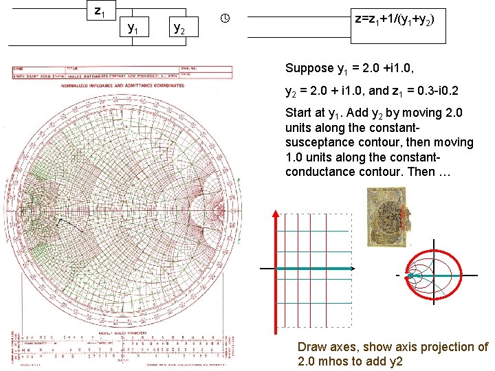
z 1 y 2 z=z 1+1/(y 1+y 2) Suppose y 1 = 2. 0 +i 1. 0, y 2 = 2. 0 + i 1. 0, and z 1 = 0. 3 -i 0. 2 Start at y 1. Add y 2 by moving 2. 0 units along the constantsusceptance contour, then moving 1. 0 units along the constantconductance contour. Then … Draw axes, y show axis projection of contours 2. 0 mhos to add y 2

z 1 y 2 z=z 1+1/(y 1+y 2) Suppose y 1 = 2. 0 +i 1. 0, y 2 = 2. 0 + i 1. 0, and z 1 = 0. 3 -i 0. 2 Start at y 1. Add y 2 by moving 2. 0 units along the constantsusceptance contour, then moving 1. 0 units along the constantconductance contour. Then … Draw axes, y show axis projection of contours i 1. 0 mhos (+y 2)

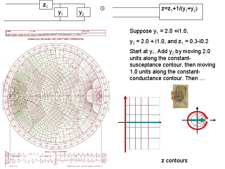
z 1 y 2 z=z 1+1/(y 1+y 2) Suppose y 1 = 2. 0 +i 1. 0, y 2 = 2. 0 + i 1. 0, and z 1 = 0. 3 -i 0. 2 Start at y 1. Add y 2 by moving 2. 0 units along the constantsusceptance contour, then moving 1. 0 units along the constantconductance contour. Then … z contours

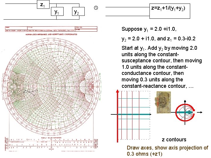
z 1 y 2 z=z 1+1/(y 1+y 2) Suppose y 1 = 2. 0 +i 1. 0, y 2 = 2. 0 + i 1. 0, and z 1 = 0. 3 -i 0. 2 Start at y 1. Add y 2 by moving 2. 0 units along the constantsusceptance contour, then moving 1. 0 units along the constantconductance contour, then moving 0. 3 units along the constant-reactance contour, … z contours Draw axes, show axis projection of 0. 3 ohms (+z 1)

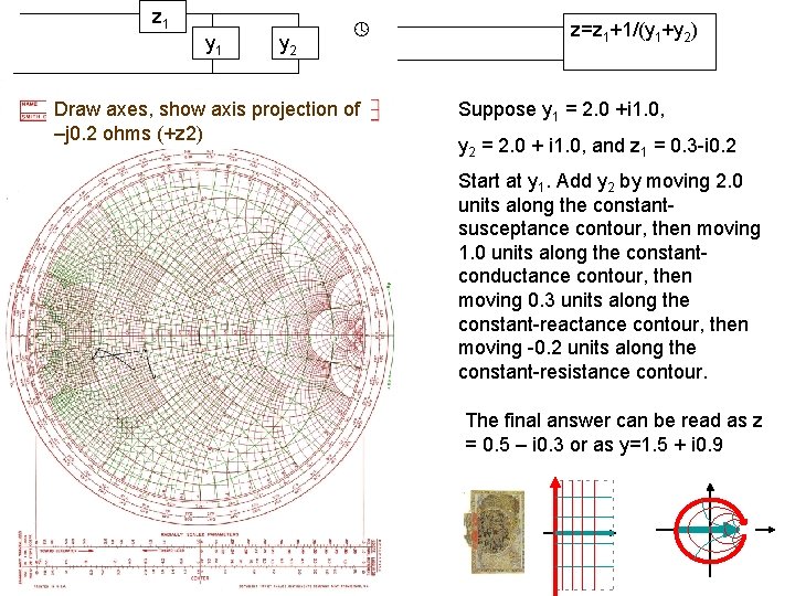
z 1 y 2 Draw axes, show axis projection of –j 0. 2 ohms (+z 2) z=z 1+1/(y 1+y 2) Suppose y 1 = 2. 0 +i 1. 0, y 2 = 2. 0 + i 1. 0, and z 1 = 0. 3 -i 0. 2 Start at y 1. Add y 2 by moving 2. 0 units along the constantsusceptance contour, then moving 1. 0 units along the constantconductance contour, then moving 0. 3 units along the constant-reactance contour, then moving -0. 2 units along the constant-resistance contour. The final answer can be read as z = 0. 5 – i 0. 3 or as y=1. 5 + i 0. 9

z 1 y 2 z=z 1+1/(y 1+y 2) Suppose y 1 = 2. 0 +i 1. 0, Read off z y 2 = 2. 0 + i 1. 0, and z 1 = 0. 3 -i 0. 2 Start at y 1. Add y 2 by moving 2. 0 units along the constantsusceptance contour, then moving 1. 0 units along the constantconductance contour, then moving 0. 3 units along the constant-reactance contour, then moving -0. 2 units along the constant-resistance contour. The final answer can be read as z = 0. 5 – i 0. 3 or as y=1. 5 + i 0. 9

z 1 y 2 z=z 1+1/(y 1+y 2) Suppose y 1 = 2. 0 +i 1. 0, Read off y y 2 = 2. 0 + i 1. 0, and z 1 = 0. 3 -i 0. 2 Start at y 1. Add y 2 by moving 2. 0 units along the constantsusceptance contour, then moving 1. 0 units along the constantconductance contour, then moving 0. 3 units along the constant-reactance contour, then moving -0. 2 units along the constant-resistance contour. The final answer can be read as z = 0. 5 – i 0. 3 or as y=1. 5 + i 0. 9

Impedance Matching

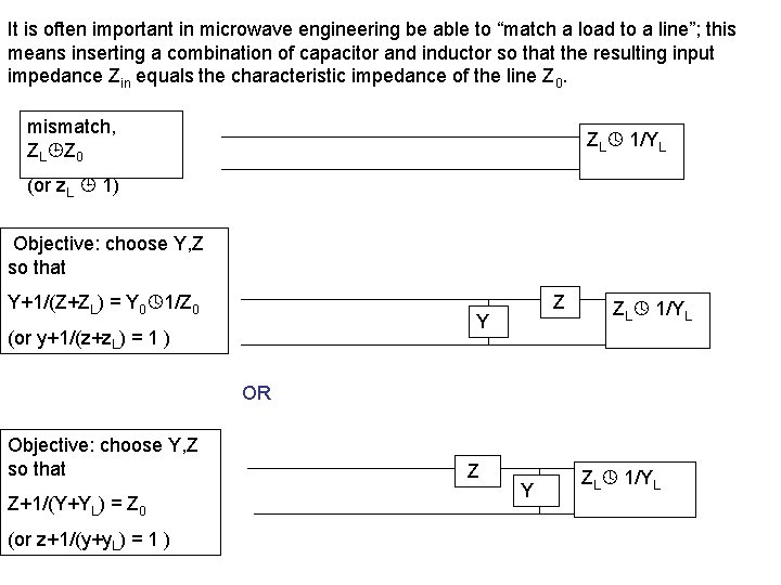
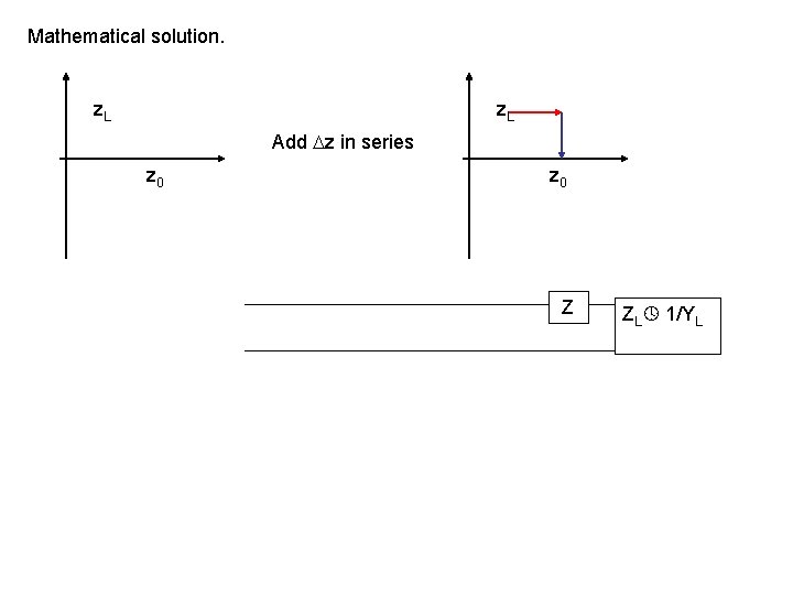
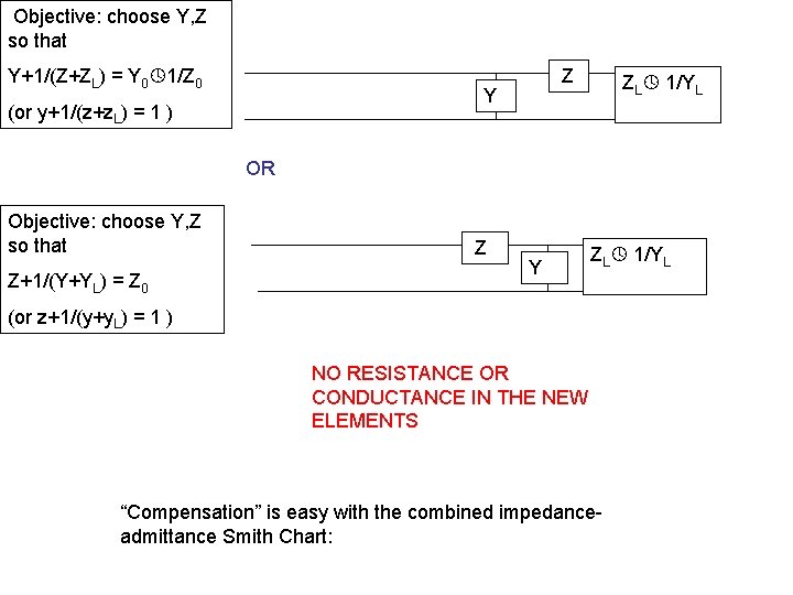
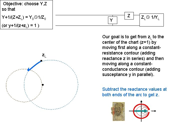
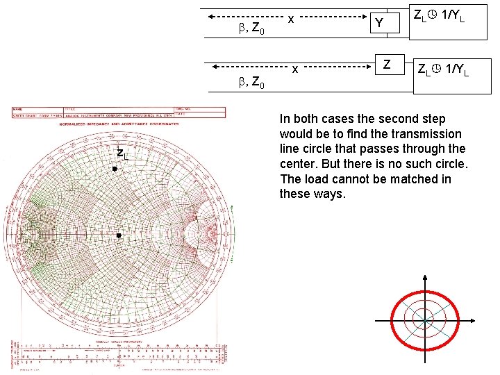
It is often important in microwave engineering be able to “match a load to a line”; this means inserting a combination of capacitor and inductor so that the resulting input impedance Zin equals the characteristic impedance of the line Z 0. mismatch, ZL Z 0 ZL 1/YL (or z. L 1) Objective: choose Y, Z so that Y+1/(Z+ZL) = Y 0 1/Z 0 Z Y (or y+1/(z+z. L) = 1 ) ZL 1/YL OR Objective: choose Y, Z so that Z+1/(Y+YL) = Z 0 (or z+1/(y+y. L) = 1 ) Z Y ZL 1/YL

Mathematical solution. z. L Add z in series z 0 Z ZL 1/YL

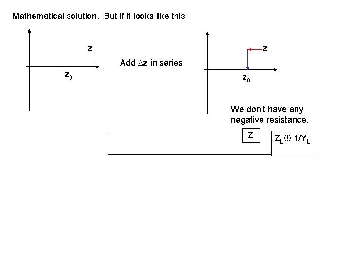
Mathematical solution. But if it looks like this z. L Add z in series z 0 We don’t have any negative resistance. Z ZL 1/YL

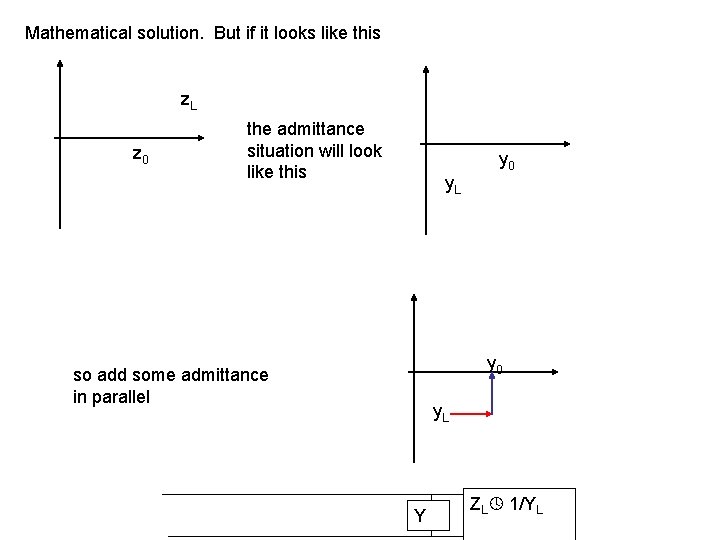
Mathematical solution. But if it looks like this z. L z 0 the admittance situation will look like this y 0 y. L y 0 so add some admittance in parallel y. L Y ZL 1/YL

For efficiency, neither Z nor Y should contain resistors. So…

Objective: choose Y, Z so that Y+1/(Z+ZL) = Y 0 1/Z 0 Z Y (or y+1/(z+z. L) = 1 ) ZL 1/YL OR Objective: choose Y, Z so that Z+1/(Y+YL) = Z 0 Z Y ZL 1/YL (or z+1/(y+y. L) = 1 ) NO RESISTANCE OR CONDUCTANCE IN THE NEW ELEMENTS “Compensation” is easy with the combined impedanceadmittance Smith Chart:

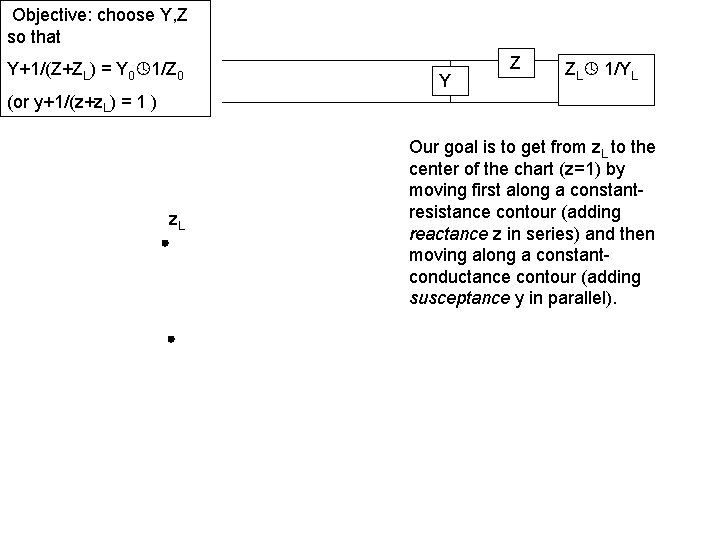
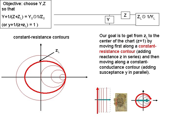
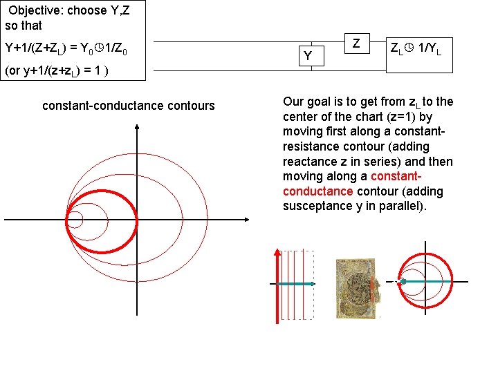
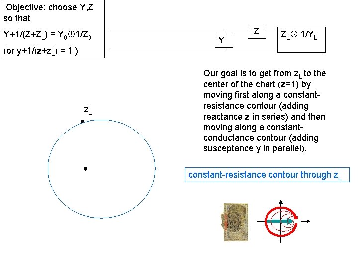
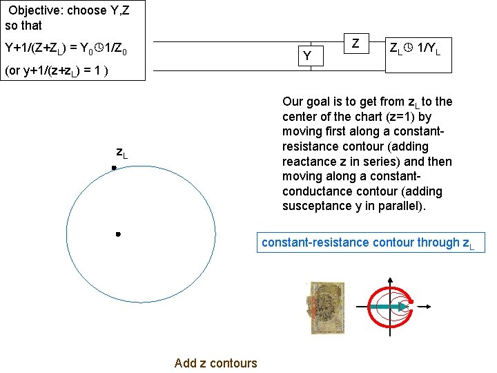
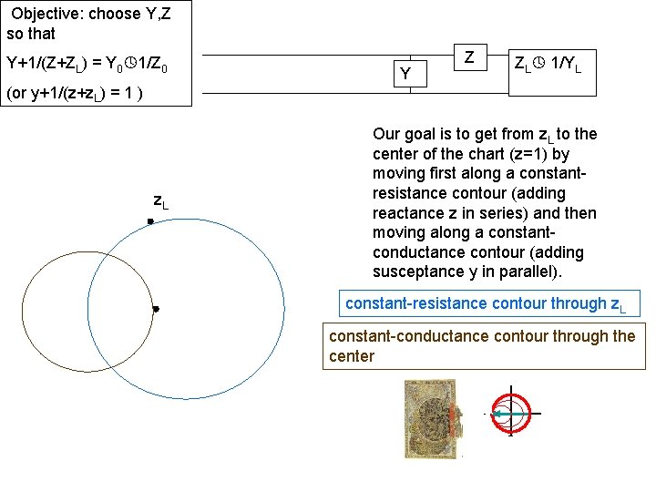
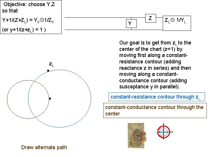
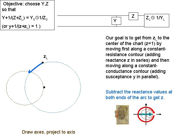
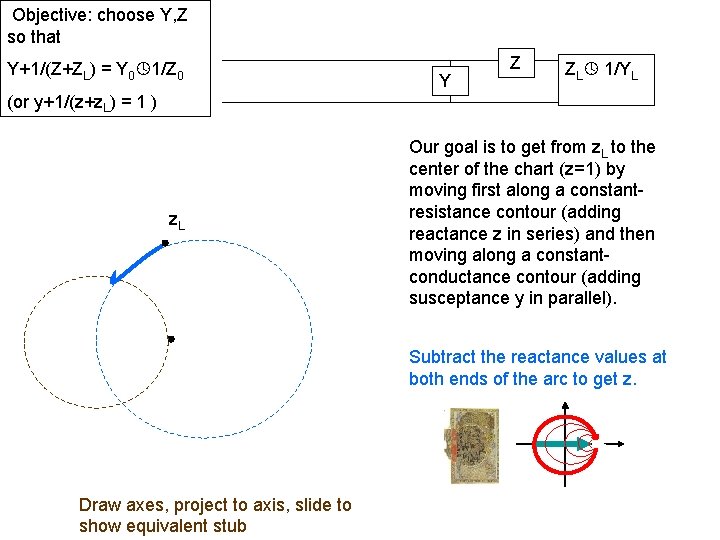
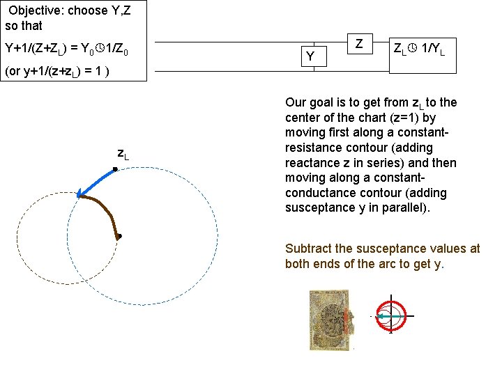
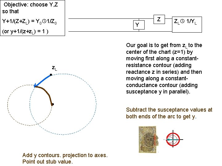
Objective: choose Y, Z so that Y+1/(Z+ZL) = Y 0 1/Z 0 Y Z ZL 1/YL (or y+1/(z+z. L) = 1 ) z. L Our goal is to get from z. L to the center of the chart (z=1) by moving first along a constantresistance contour (adding reactance z in series) and then moving along a constantconductance contour (adding susceptance y in parallel).

Objective: choose Y, Z so that Y+1/(Z+ZL) = Y 0 1/Z 0 Y Z ZL 1/YL (or y+1/(z+z. L) = 1 ) constant-resistance contours z. L Our goal is to get from z. L to the center of the chart (z=1) by moving first along a constantresistance contour (adding reactance z in series) and then moving along a constantconductance contour (adding susceptance y in parallel).

Objective: choose Y, Z so that Y+1/(Z+ZL) = Y 0 1/Z 0 Y Z ZL 1/YL (or y+1/(z+z. L) = 1 ) constant-conductance contours Our goal is to get from z. L to the center of the chart (z=1) by moving first along a constantresistance contour (adding reactance z in series) and then moving along a constantconductance contour (adding susceptance y in parallel).

Objective: choose Y, Z so that Y+1/(Z+ZL) = Y 0 1/Z 0 Y Z ZL 1/YL (or y+1/(z+z. L) = 1 ) z. L Our goal is to get from z. L to the center of the chart (z=1) by moving first along a constantresistance contour (adding reactance z in series) and then moving along a constantconductance contour (adding susceptance y in parallel). constant-resistance contour through z. L

Objective: choose Y, Z so that Y+1/(Z+ZL) = Y 0 1/Z 0 Y Z ZL 1/YL (or y+1/(z+z. L) = 1 ) Our goal is to get from z. L to the center of the chart (z=1) by moving first along a constantresistance contour (adding reactance z in series) and then moving along a constantconductance contour (adding susceptance y in parallel). z. L constant-resistance contour through z. L Add z contours

Objective: choose Y, Z so that Y+1/(Z+ZL) = Y 0 1/Z 0 Y Z ZL 1/YL (or y+1/(z+z. L) = 1 ) z. L Our goal is to get from z. L to the center of the chart (z=1) by moving first along a constantresistance contour (adding reactance z in series) and then moving along a constantconductance contour (adding susceptance y in parallel). constant-resistance contour through z. L constant-conductance contour through the center

Objective: choose Y, Z so that Y+1/(Z+ZL) = Y 0 1/Z 0 Y Z ZL 1/YL (or y+1/(z+z. L) = 1 ) z. L Our goal is to get from z. L to the center of the chart (z=1) by moving first along a constantresistance contour (adding reactance z in series) and then moving along a constantconductance contour (adding susceptance y in parallel). constant-resistance contour through z. L constant-conductance contour through the center Draw alternate path

Objective: choose Y, Z so that Y+1/(Z+ZL) = Y 0 1/Z 0 Y Z ZL 1/YL (or y+1/(z+z. L) = 1 ) z. L Our goal is to get from z. L to the center of the chart (z=1) by moving first along a constantresistance contour (adding reactance z in series) and then moving along a constantconductance contour (adding susceptance y in parallel). Subtract the reactance values at both ends of the arc to get z.

Objective: choose Y, Z so that Y+1/(Z+ZL) = Y 0 1/Z 0 Y Z ZL 1/YL (or y+1/(z+z. L) = 1 ) z. L Our goal is to get from z. L to the center of the chart (z=1) by moving first along a constantresistance contour (adding reactance z in series) and then moving along a constantconductance contour (adding susceptance y in parallel). Subtract the reactance values at both ends of the arc to get z. Draw axes, project to axis

Objective: choose Y, Z so that Y+1/(Z+ZL) = Y 0 1/Z 0 Y Z ZL 1/YL (or y+1/(z+z. L) = 1 ) z. L Our goal is to get from z. L to the center of the chart (z=1) by moving first along a constantresistance contour (adding reactance z in series) and then moving along a constantconductance contour (adding susceptance y in parallel). Subtract the reactance values at both ends of the arc to get z. Draw axes, project to axis, slide to show equivalent stub

Objective: choose Y, Z so that Y+1/(Z+ZL) = Y 0 1/Z 0 Y Z ZL 1/YL (or y+1/(z+z. L) = 1 ) z. L Our goal is to get from z. L to the center of the chart (z=1) by moving first along a constantresistance contour (adding reactance z in series) and then moving along a constantconductance contour (adding susceptance y in parallel). Subtract the susceptance values at both ends of the arc to get y.

Objective: choose Y, Z so that Y+1/(Z+ZL) = Y 0 1/Z 0 Y Z ZL 1/YL (or y+1/(z+z. L) = 1 ) z. L Our goal is to get from z. L to the center of the chart (z=1) by moving first along a constantresistance contour (adding reactance z in series) and then moving along a constantconductance contour (adding susceptance y in parallel). Subtract the susceptance values at both ends of the arc to get y. Add y contours. projection to axes. Point out stub value.

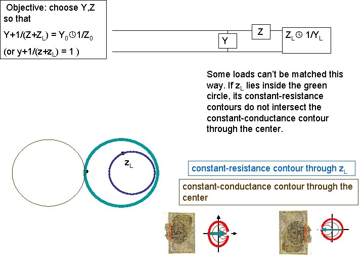
Objective: choose Y, Z so that Y+1/(Z+ZL) = Y 0 1/Z 0 Y Z ZL 1/YL (or y+1/(z+z. L) = 1 ) Some loads can’t be matched this way. If z. L lies inside the green circle, its constant-resistance contours do not intersect the constant-conductance contour through the center. z. L constant-resistance contour through z. L constant-conductance contour through the center

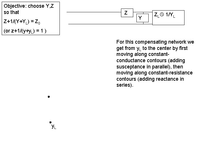
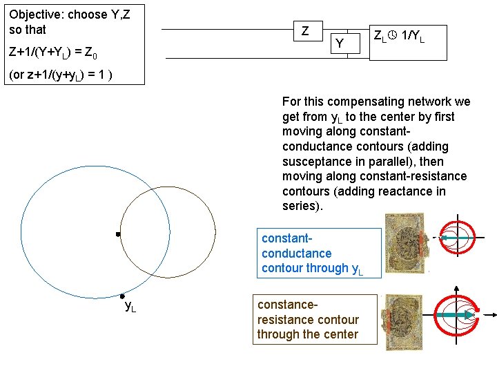
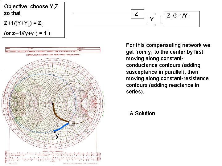
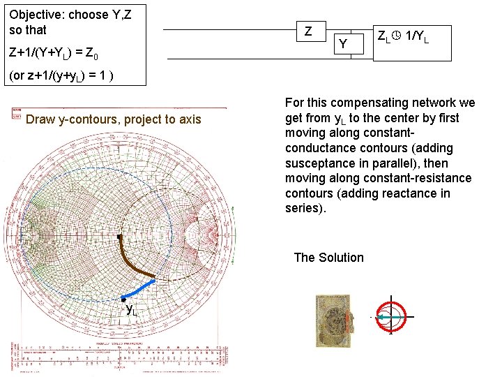
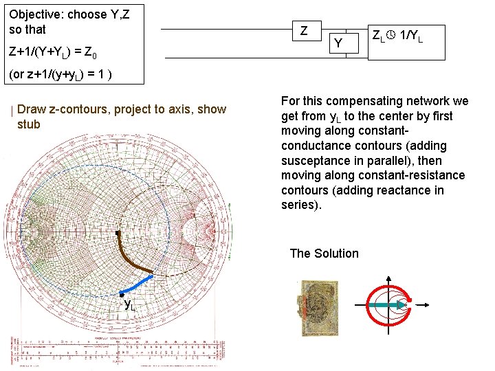
Objective: choose Y, Z so that Z+1/(Y+YL) = Z 0 Z Y ZL 1/YL (or z+1/(y+y. L) = 1 ) For this compensating network we get from y. L to the center by first moving along constantconductance contours (adding susceptance in parallel), then moving along constant-resistance contours (adding reactance in series). y. L

Objective: choose Y, Z so that Z+1/(Y+YL) = Z 0 Z Y ZL 1/YL (or z+1/(y+y. L) = 1 ) For this compensating network we get from y. L to the center by first moving along constantconductance contours (adding susceptance in parallel), then moving along constant-resistance contours (adding reactance in series). constantconductance contour through y. L constanceresistance contour through the center

Objective: choose Y, Z so that Z+1/(Y+YL) = Z 0 Z Y ZL 1/YL (or z+1/(y+y. L) = 1 ) For this compensating network we get from y. L to the center by first moving along constantconductance contours (adding susceptance in parallel), then moving along constant-resistance contours (adding reactance in series). A Solution y. L

Objective: choose Y, Z so that Z+1/(Y+YL) = Z 0 Z Y ZL 1/YL (or z+1/(y+y. L) = 1 ) Draw y-contours, project to axis For this compensating network we get from y. L to the center by first moving along constantconductance contours (adding susceptance in parallel), then moving along constant-resistance contours (adding reactance in series). The Solution y. L

Objective: choose Y, Z so that Z+1/(Y+YL) = Z 0 Z Y ZL 1/YL (or z+1/(y+y. L) = 1 ) Draw z-contours, project to axis, show stub For this compensating network we get from y. L to the center by first moving along constantconductance contours (adding susceptance in parallel), then moving along constant-resistance contours (adding reactance in series). The Solution y. L

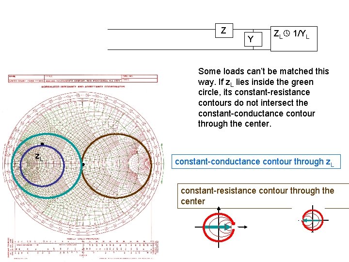
Z Y ZL 1/YL Some loads can’t be matched this way. If z. L lies inside the green circle, its constant-resistance contours do not intersect the constant-conductance contour through the center. z. L constant-conductance contour through z. L constant-resistance contour through the center

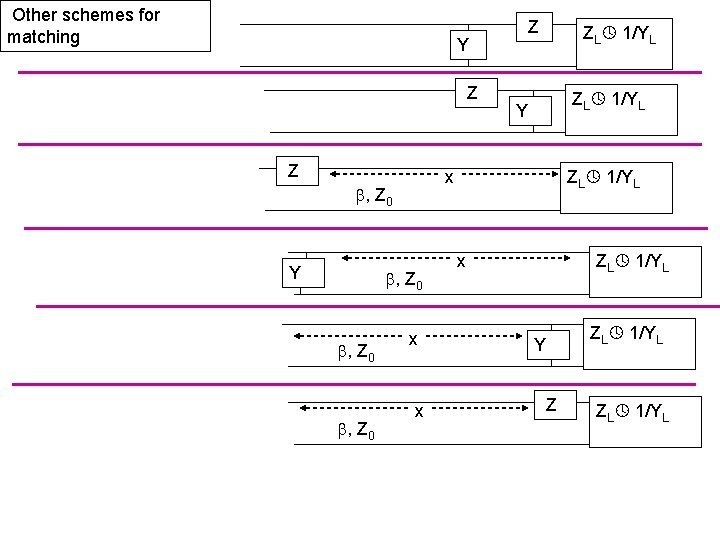
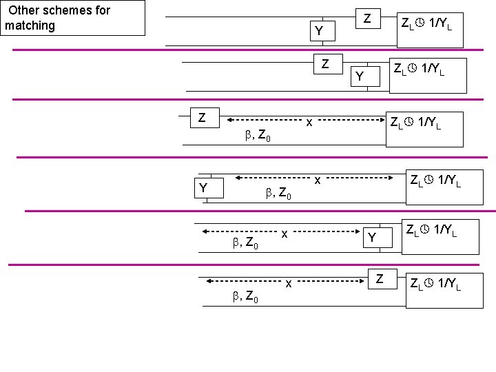
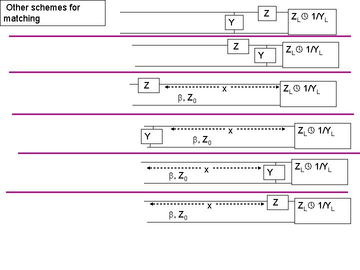
Other schemes for matching Y Z Z , Z 0 ZL 1/YL Y ZL 1/YL x , Z 0 Y Z x x ZL 1/YL x Y Z ZL 1/YL

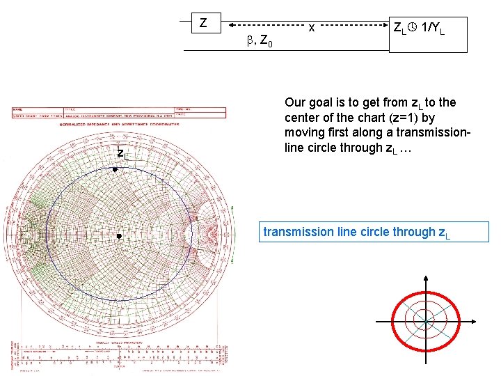
Z , Z 0 z. L x ZL 1/YL Our goal is to get from z. L to the center of the chart (z=1) by moving first along a transmissionline circle through z. L … transmission line circle through z. L

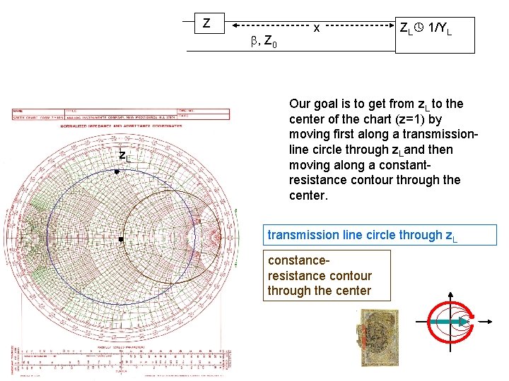
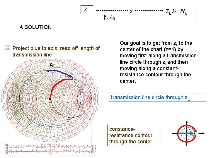
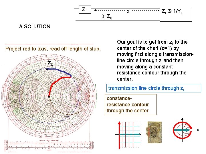
Z , Z 0 z. L x ZL 1/YL Our goal is to get from z. L to the center of the chart (z=1) by moving first along a transmissionline circle through z. Land then moving along a constantresistance contour through the center. transmission line circle through z. L constanceresistance contour through the center

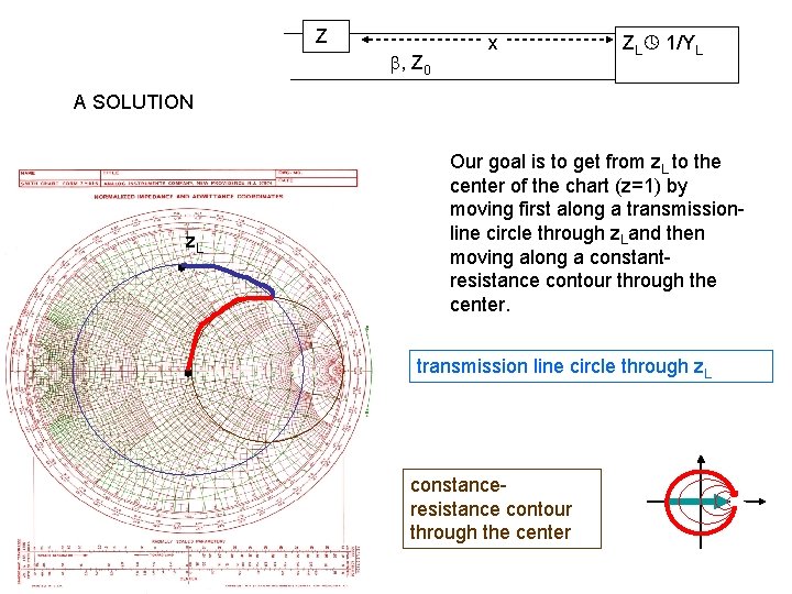
Z , Z 0 x ZL 1/YL A SOLUTION z. L Our goal is to get from z. L to the center of the chart (z=1) by moving first along a transmissionline circle through z. Land then moving along a constantresistance contour through the center. transmission line circle through z. L constanceresistance contour through the center

Z , Z 0 x ZL 1/YL A SOLUTION Project blue to axis, read off length of transmission line z. L Our goal is to get from z. L to the center of the chart (z=1) by moving first along a transmissionline circle through z. Land then moving along a constantresistance contour through the center. transmission line circle through z. L constanceresistance contour through the center

Z , Z 0 x ZL 1/YL A SOLUTION Project red to axis, read off length of stub. z. L Our goal is to get from z. L to the center of the chart (z=1) by moving first along a transmissionline circle through z. Land then moving along a constantresistance contour through the center. transmission line circle through z. L constanceresistance contour through the center

Other schemes for matching Y Z Z , Z 0 ZL 1/YL Y ZL 1/YL x , Z 0 Y Z x x ZL 1/YL x Y Z ZL 1/YL

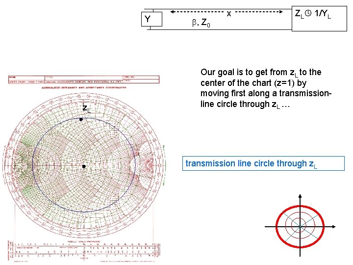
Y z. L , Z 0 x ZL 1/YL Our goal is to get from z. L to the center of the chart (z=1) by moving first along a transmissionline circle through z. L … transmission line circle through z. L

Y z. L , Z 0 x ZL 1/YL Our goal is to get from z. L to the center of the chart (z=1) by moving first along a transmissionline circle through z. Land then moving along a constantconductance contour through the center. transmission line circle through z. L constanceconductance contour through the center

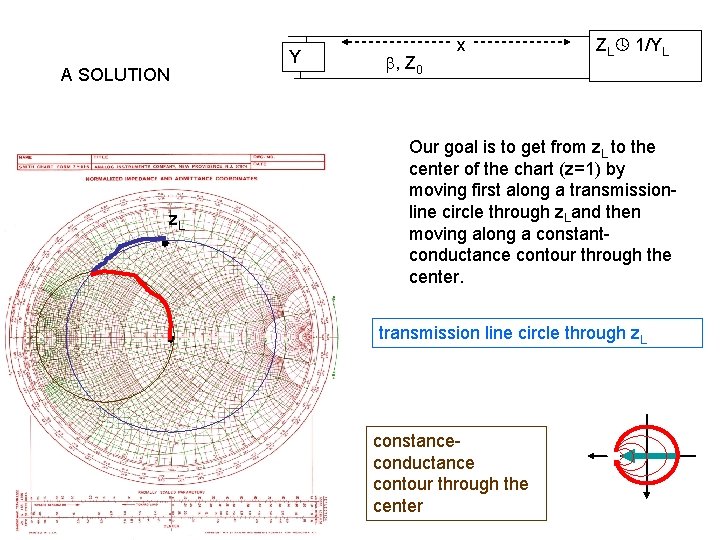
A SOLUTION z. L Y , Z 0 x ZL 1/YL Our goal is to get from z. L to the center of the chart (z=1) by moving first along a transmissionline circle through z. Land then moving along a constantconductance contour through the center. transmission line circle through z. L constanceconductance contour through the center

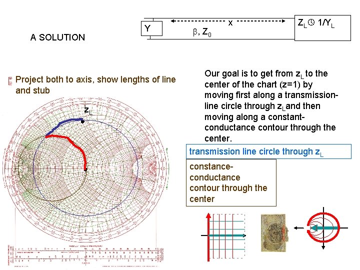
A SOLUTION Y Project both to axis, show lengths of line and stub z. L , Z 0 x ZL 1/YL Our goal is to get from z. L to the center of the chart (z=1) by moving first along a transmissionline circle through z. Land then moving along a constantconductance contour through the center. transmission line circle through z. L constanceconductance contour through the center

Other schemes for matching Y Z Z , Z 0 ZL 1/YL Y ZL 1/YL x , Z 0 Y Z x x ZL 1/YL x Y Z ZL 1/YL

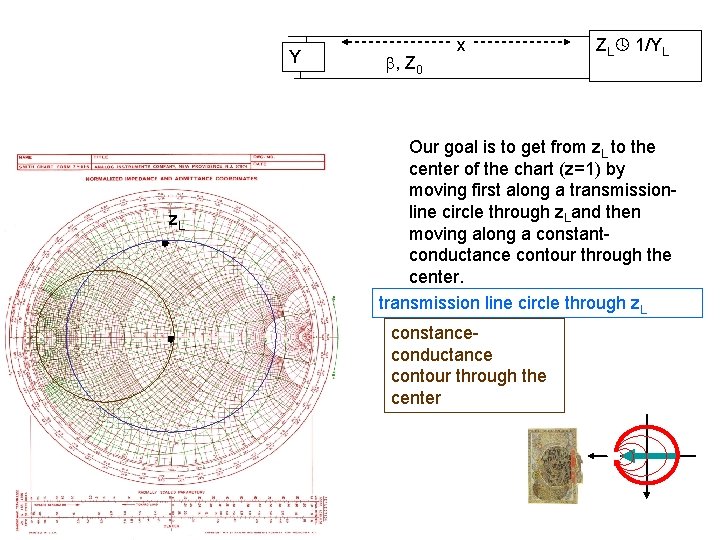
, Z 0 z. L x x Y Z ZL 1/YL In both cases the second step would be to find the transmission line circle that passes through the center. But there is no such circle. The load cannot be matched in these ways.

NOISE PARAMETERS

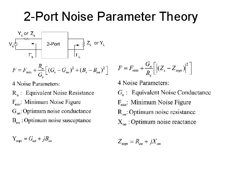
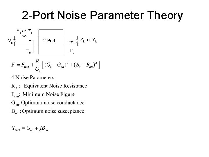
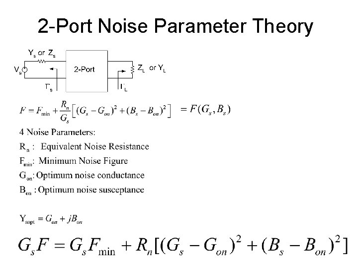
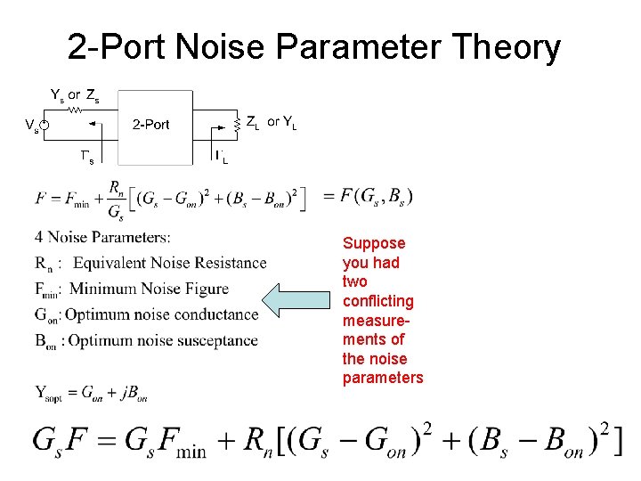
2 -Port Noise Parameter Theory

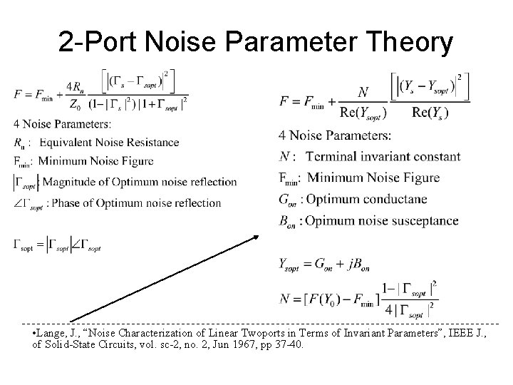
2 -Port Noise Parameter Theory • Lange, J. , “Noise Characterization of Linear Twoports in Terms of Invariant Parameters”, IEEE J. , of Solid-State Circuits, vol. sc-2, no. 2, Jun 1967, pp 37 -40.

2 -Port Noise Parameter Theory

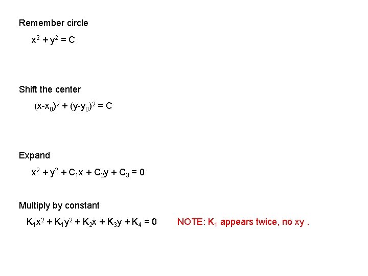
Remember circle x 2 + y 2 = C Shift the center (x-x 0)2 + (y-y 0)2 = C Expand x 2 + y 2 + C 1 x + C 2 y + C 3 = 0 Multiply by constant K 1 x 2 + K 1 y 2 + K 2 x + K 3 y + K 4 = 0 NOTE: K 1 appears twice, no xy.

2 -Port Noise Parameter Theory

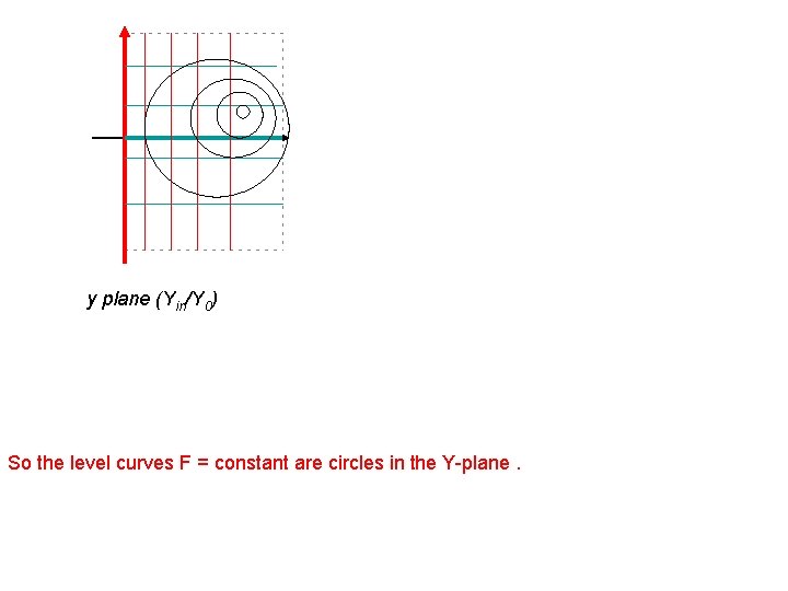
y plane (Yin/Y 0) So the level curves F = constant are circles in the Y-plane.

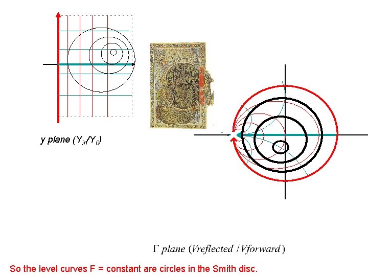
y plane (Yin/Y 0) Lines-and-circles go to lines-and-circles

y plane (Yin/Y 0) So the level curves F = constant are circles in the Smith disc.

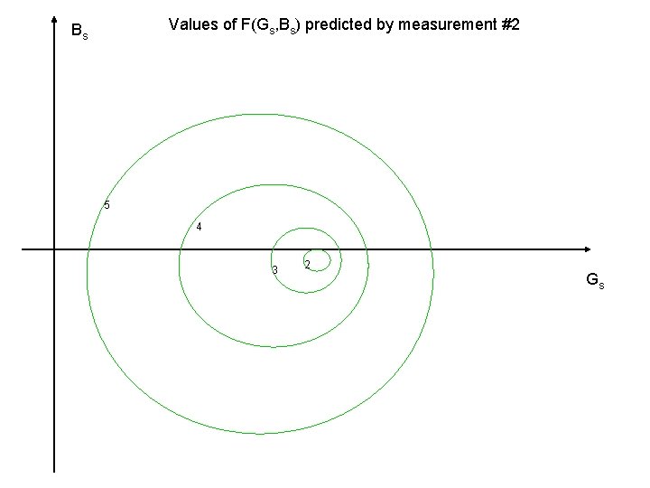
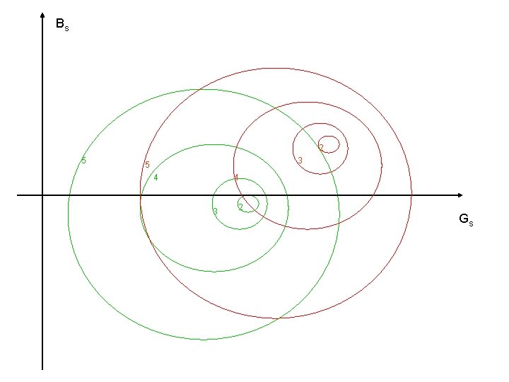
2 -Port Noise Parameter Theory Suppose you had two conflicting measurements of the noise parameters

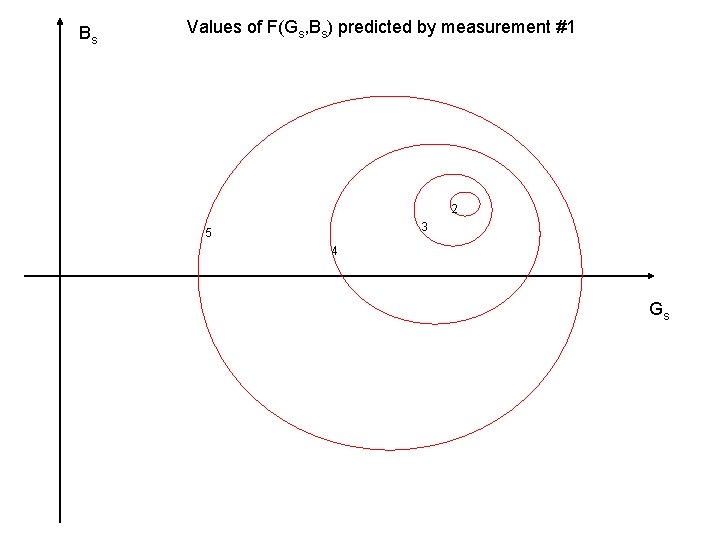
Bs Values of F(Gs, Bs) predicted by measurement #1 2 3 5 4 Gs

Values of F(Gs, Bs) predicted by measurement #2 Bs 5 4 3 2 Gs

Bs 2 5 3 5 4 4 3 2 Gs

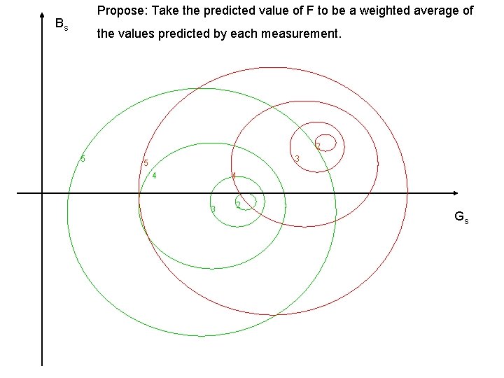
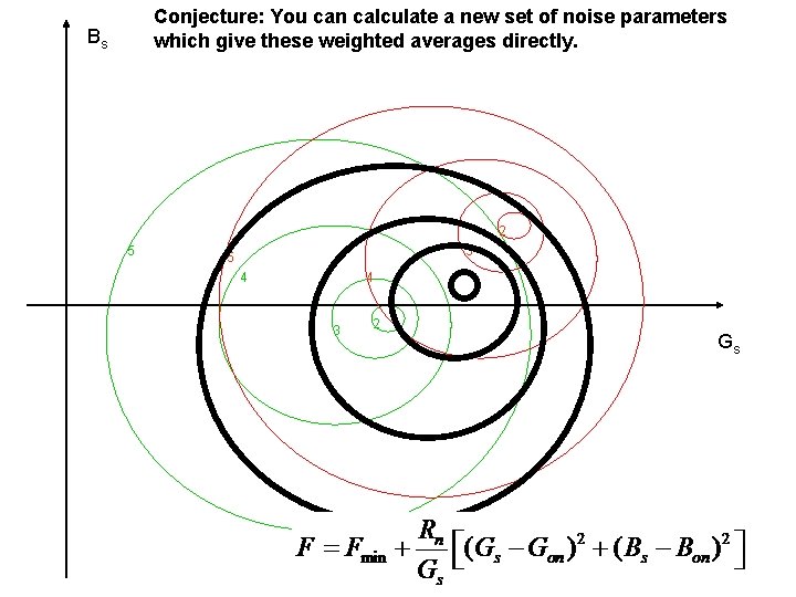
Propose: Take the predicted value of F to be a weighted average of Bs the values predicted by each measurement. 2 5 3 5 4 4 3 2 Gs

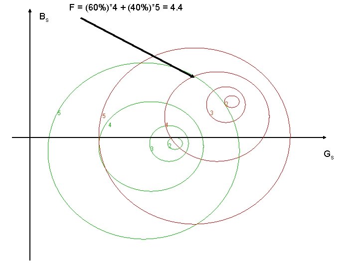
F = (60%)*4 + (40%)*5 = 4. 4 Bs 2 5 3 5 4 4 3 2 Gs

Conjecture: You can calculate a new set of noise parameters which give these weighted averages directly. Bs 2 5 3 5 4 4 3 2 Gs