Sliding Window Filters and Edge Detection Longin Jan

Sliding Window Filters and Edge Detection Longin Jan Latecki Computer Graphics and Image Processing CIS 601 – Fall 2003

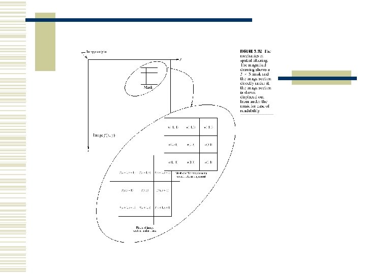
Linear Image Filters Linear operations calculate the resulting value in the output image pixel f(i, j) as a linear combination of brightness in a local neighborhood of the pixel h(i, j) in the input image. This equation is called to discrete convolution: Function w is called a convolution kernel or a filter mask. In our case it is a rectangle of size (2 a+1)x(2 b+1).

Exercise: Compute the 2 -D linear convolution of the following two signal X with mask w. Extend the signal X with 0’s where needed.

Image smoothing = image blurring Averaging of brightness values is a special case of discrete convolution. For a 3 x 3 neighborhood the convolution mask w is Applying this mask to an image results in smoothing. Matlab example program is filter. Ex 1. m • Local image smoothing can effectively eliminate impulsive noise or degradations appearing as thin stripes, but does not work if degradations are large blobs or thick stripes.

The significance of the central pixel may be increased to better reflect properties of Gaussian noise:

Nonlinear Image Filters Median is an order filter, it uses order statistics. Given an Nx. N window W(x, y) with pixel (x, y) being the midpoint of W, the pixel intensity values of pixels in W are ordered from smallest to the largest, as follow: Median filter selects the middle value as the value of (x, y).

Morphological Filters

For comparison see Order Filters on www. ee. siue. edu/~cvip/CVIPtools_demos/mainframe. shtml Homework Implement in Matlab a linear filter for image smoothing (blurring) using convolution method (filter 2 function). Implement alos nonlinear filters: median, opening, and closing (simply using two for loops). Apply them to images noise_1. gif, noise_2. gif in www. cis. temple. edu/~latecki/CIS 601 -03LecturesMatlabImages Compare the results.

Edge Detection • What are edges in an image? • Edge Detection Methods • Edge Operators • Matlab Program • Performance

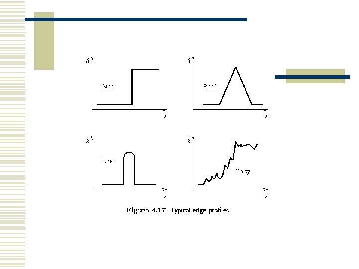
What are edges in an image? w Edges are those places in an image that correspond to object boundaries. w Edges are pixels where image brightness changes abruptly. Brightness vs. Spatial Coordinates

More About Edges w An edge is a property attached to an individual pixel and is calculated from the image function behavior in a neighborhood of the pixel. w It is a vector variable (magnitude of the gradient, direction of an edge).

Image To Edge Map

Edge Detection w Edge information in an image is found by looking at the relationship a pixel has with its neighborhoods. w If a pixel’s gray-level value is similar to those around it, there is probably not an edge at that point. w If a pixel’s has neighbors with widely varying gray levels, it may present an edge point.

Edge Detection Methods w Many are implemented with convolution mask and based on discrete approximations to differential operators. w Differential operations measure the rate of change in the image brightness function. w Some operators return orientation information. Other only return information about the existence of an edge at each point.

A 2 D grayvalue - image is a 2 D -> 1 D function v = f(x, y)

Edge detectors • locate sharp changes in the intensity function • edges are pixels where brightness changes abruptly. • Calculus describes changes of continuous functions using derivatives; an image function depends on two variables - partial derivatives. • A change of the image function can be described by a gradient that points in the direction of the largest growth of the image function. • An edge is a property attached to an individual pixel and is calculated from the image function behavior in a neighborhood of the pixel. • It is a vector variable: magnitude of the gradient and direction

• The gradient direction gives the direction of maximal growth of the function, e. g. , from black (f(i, j)=0) to white (f(i, j)=255). • This is illustrated below; closed lines are lines of the same brightness. • Boundary and its parts (edges) are perpendicular to the direction of the gradient.

• The gradient magnitude and gradient direction are continuous image functions, where arg(x, y) is the angle (in radians) from the x-axis to the point (x, y).

• A digital image is discrete in nature, derivatives must be approximated by differences. • The first differences of the image g in the vertical direction (for fixed i) and in the horizontal direction (for fixed j) • n is a small integer, usually 1. The value n should be chosen small enough to provide a good approximation to the derivative, but large enough to neglect unimportant changes in the image function.

Roberts Operator w Mark edge point only w No information about edge orientation w Work best with binary images w Primary disadvantage: n n High sensitivity to noise Few pixels are used to approximate the gradient

Roberts Operator (Cont. ) w First form of Roberts Operator w Second form of Roberts Operator

Prewitt Operator w Looks for edges in both horizontal and vertical directions, then combine the information into a single metric. Edge Magnitude = Edge Direction =

Sobel Operator w Similar to the Prewitt, with different mask coefficients: Edge Magnitude = Edge Direction =

Kirsch Compass Masks w Taking a single mask and rotating it to 8 major compass orientations: N, NW, W, SW, S, SE, E, and NE. w The edge magnitude = The maximum value found by the convolution of each mask with the image. w The edge direction is defined by the mask that produces the maximum magnitude.

Kirsch Compass Masks (Cont. ) w The Kirsch masks are defined as follows: w EX: If NE produces the maximum value, then the edge direction is Northeast

Robinson Compass Masks w Similar to the Kirsch masks, with mask coefficients of 0, 1, and 2:

• Sometimes we are interested only in edge magnitudes without regard to their orientations. • The Laplacian may be used. • The Laplacian has the same properties in all directions and is therefore invariant to rotation in the image. • The Laplace operator is a very popular operator approximating the second derivative which gives the gradient magnitude only.

Laplacian Operators w Edge magnitude is approximated in digital images by a convolution sum. w The sign of the result (+ or -) from two adjacent pixels provide edge orientation and tells us which side of edge brighter

Laplacian Operators (Cont. ) w Masks for 4 and 8 neighborhoods w Mask with stressed significance of the central pixel or its neighborhood

Performance w Please try the following link Matlab demo. To run type EDgui w Sobel and Prewitt methods are very effectively providing good edge maps. w Kirsch and Robinson methods require more time for calculation and their results are not better than the ones produced by Sobel and Prewitt methods. w Roberts and Laplacian methods are not very good as expected.

• Gradient operators can be divided into three categories I. Operators approximating derivatives of the image function using differences. • rotationally invariant (e. g. , Laplacian) need one convolution mask only. Individual gradient operators that examine small local neighborhoods are in fact convolutions and can be expressed by convolution masks. • approximating first derivatives use several masks, the orientation is estimated on the basis of the best matching of several simple patterns. Operators which are able to detect edge direction. Each mask corresponds to a certain direction.

II. Operators based on the zero crossings of the image function second derivative (e. g. , Marr-Hildreth or Canny edge detector). III. Operators which attempt to match an image function to a parametric model of edges. Parametric models describe edges more precisely than simple edge magnitude and direction and are much more computationally intensive. The categories II and III will not be covered here;

A Quick Note w Matlab’s image processing toolbox provides edge function to find edges in an image: I = imread('rice. tif'); BW 1 = edge(I, 'prewitt'); BW 2 = edge(I, 'canny'); imshow(BW 1) figure, imshow(BW 2) w Edge function supports six different edge-finding methods: Sobel, Prewitt, Roberts, Laplacian of Gaussian, Zero-cross, and Canny.

Homework: Edge Map in Matlab w Select an example image. w Which of the six edge detection method provided by Matlab works best for you. w Show the result of edge map