Slides for the book Probabilistic Robotics Authors Sebastian

Slides for the book: Probabilistic Robotics • Authors: • Sebastian Thrun • Wolfram Burgard • Dieter Fox • Publisher: • MIT Press, 2005. • Web site for the book & more slides: http: //www. probabilistic-robotics. org/ 1

Probabilistic Robotics Bayes Filter Implementations Gaussian filters 2

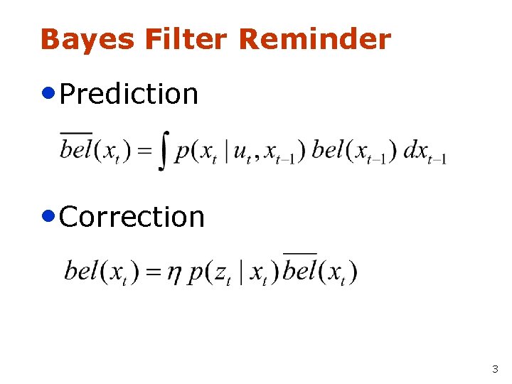
Bayes Filter Reminder • Prediction • Correction 3

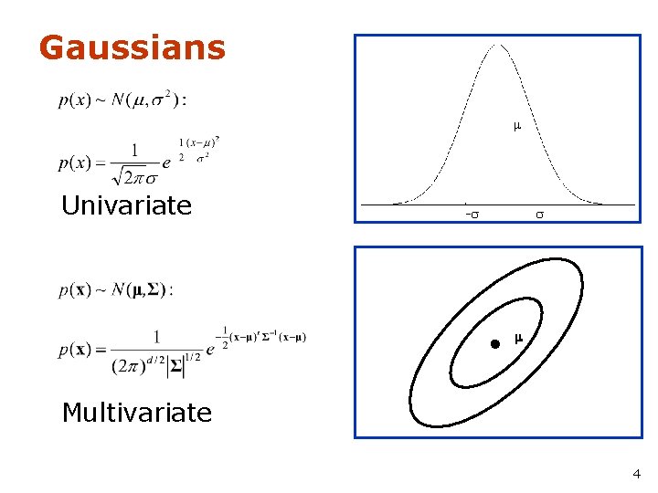
Gaussians m Univariate -s s m Multivariate 4

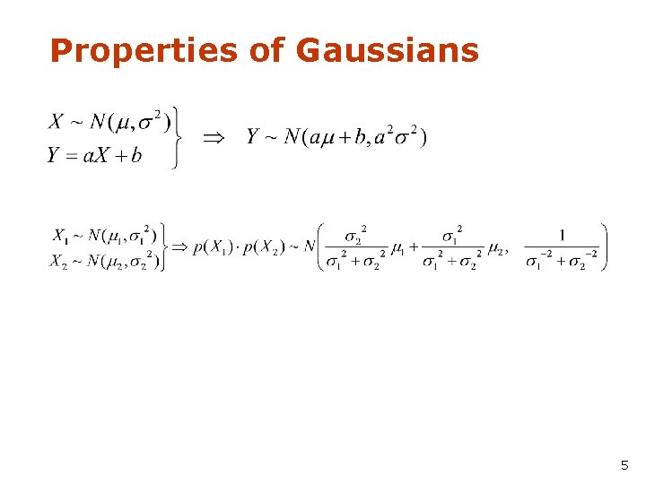
Properties of Gaussians 5

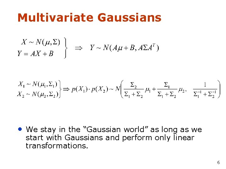
Multivariate Gaussians • We stay in the “Gaussian world” as long as we start with Gaussians and perform only linear transformations. 6

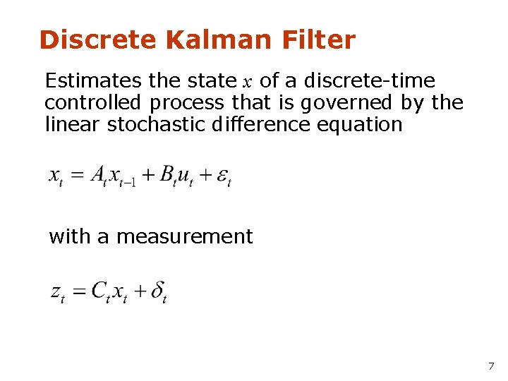
Discrete Kalman Filter Estimates the state x of a discrete-time controlled process that is governed by the linear stochastic difference equation with a measurement 7

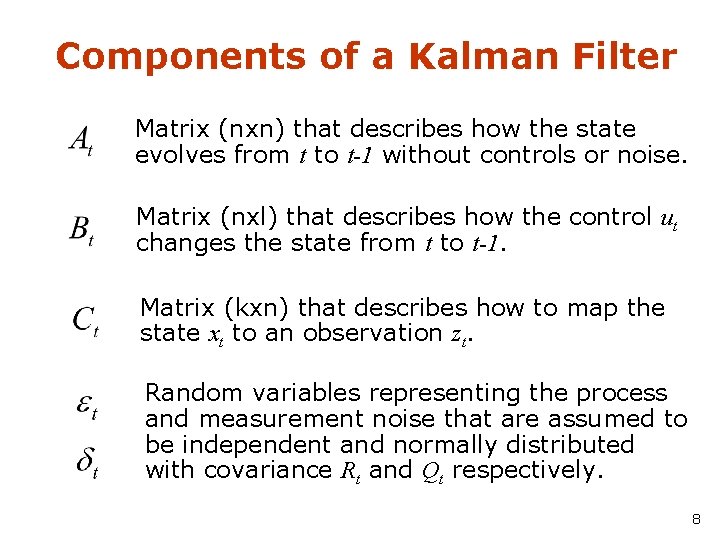
Components of a Kalman Filter Matrix (nxn) that describes how the state evolves from t to t-1 without controls or noise. Matrix (nxl) that describes how the control ut changes the state from t to t-1. Matrix (kxn) that describes how to map the state xt to an observation zt. Random variables representing the process and measurement noise that are assumed to be independent and normally distributed with covariance Rt and Qt respectively. 8

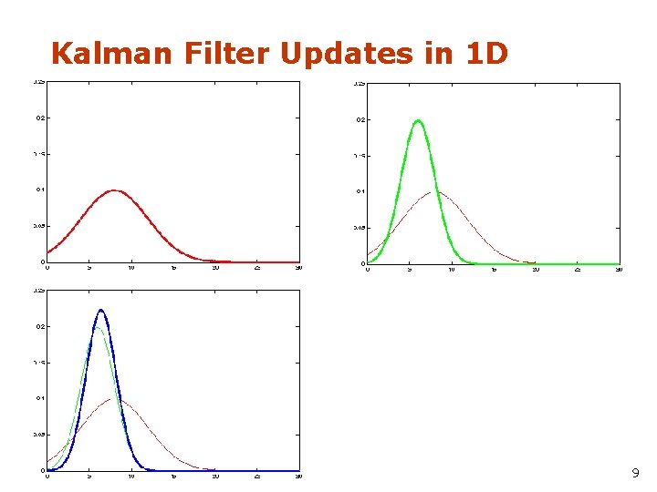
Kalman Filter Updates in 1 D 9

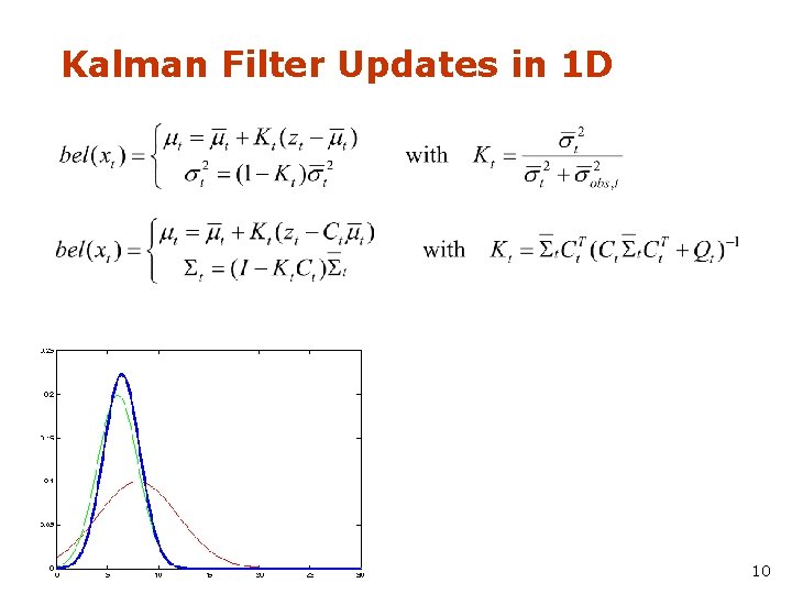
Kalman Filter Updates in 1 D 10

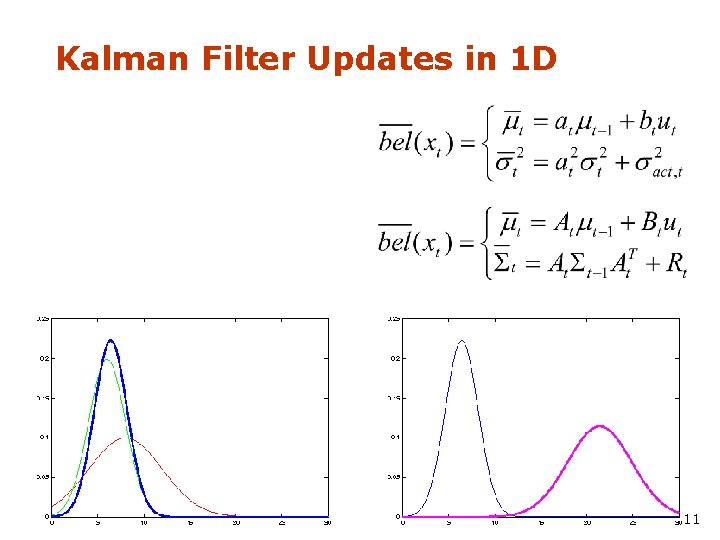
Kalman Filter Updates in 1 D 11

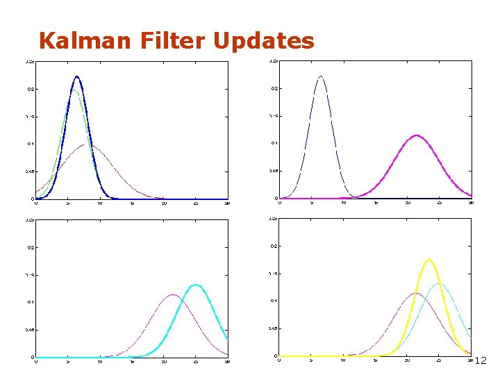
Kalman Filter Updates 12

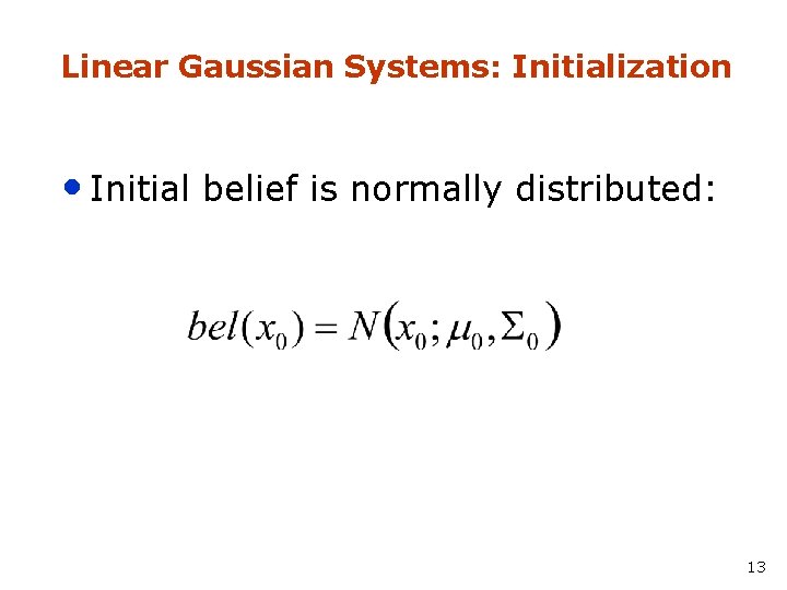
Linear Gaussian Systems: Initialization • Initial belief is normally distributed: 13

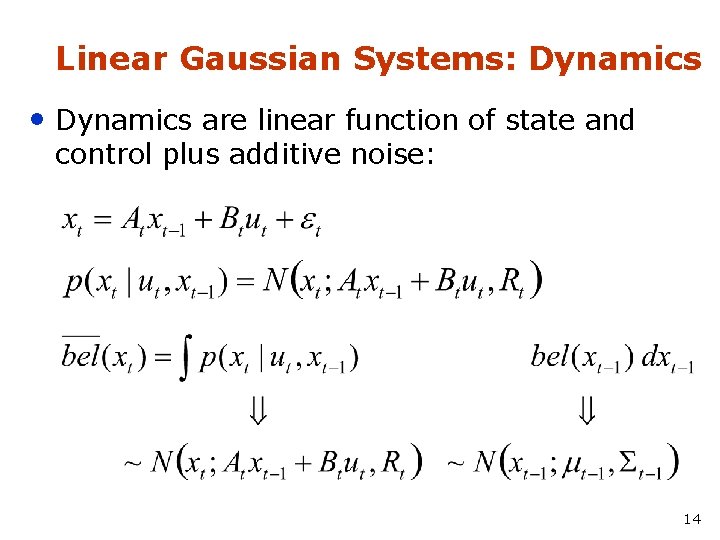
Linear Gaussian Systems: Dynamics • Dynamics are linear function of state and control plus additive noise: 14

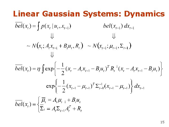
Linear Gaussian Systems: Dynamics 15

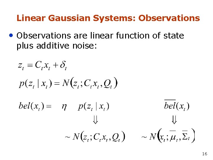
Linear Gaussian Systems: Observations • Observations are linear function of state plus additive noise: 16

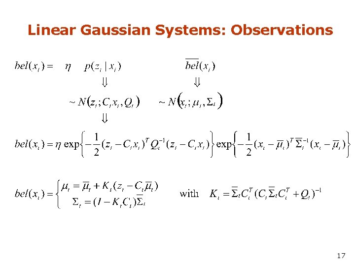
Linear Gaussian Systems: Observations 17

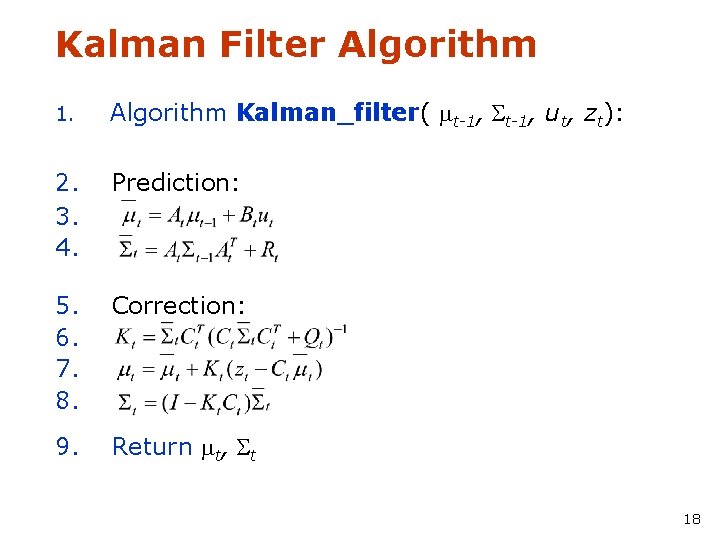
Kalman Filter Algorithm 1. Algorithm Kalman_filter( mt-1, St-1, ut, zt): 2. 3. 4. Prediction: 5. 6. 7. 8. Correction: 9. Return mt, St 18

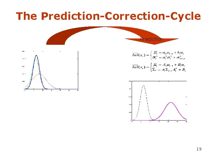
The Prediction-Correction-Cycle Prediction 19

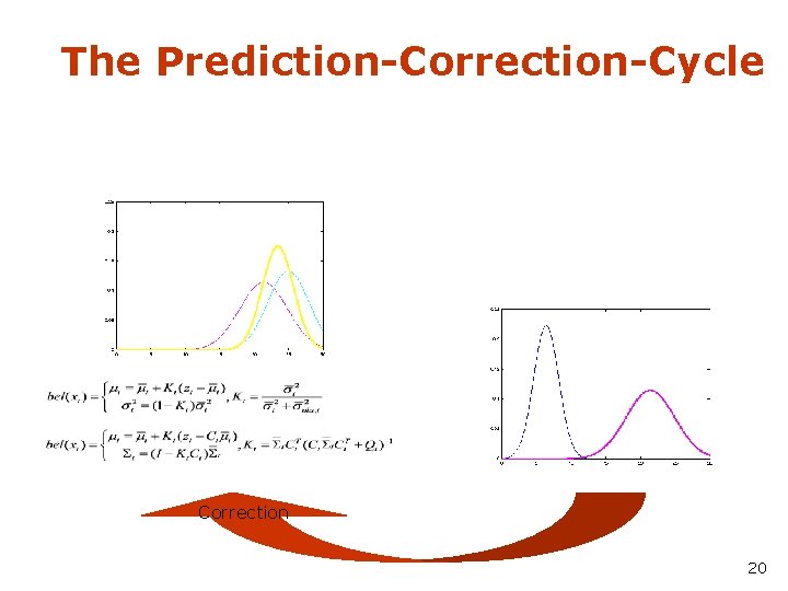
The Prediction-Correction-Cycle Correction 20

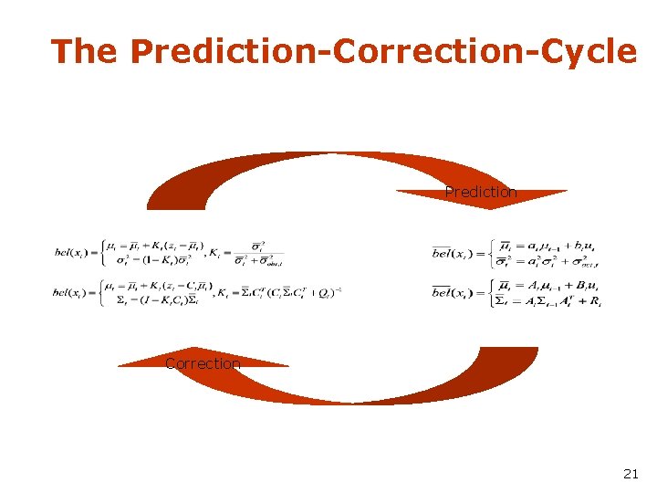
The Prediction-Correction-Cycle Prediction Correction 21

Kalman Filter Summary • Highly efficient: Polynomial in measurement dimensionality k and state dimensionality n: O(k 2. 376 + n 2) • Optimal for linear Gaussian systems! • Most robotics systems are nonlinear! 22

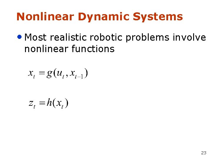
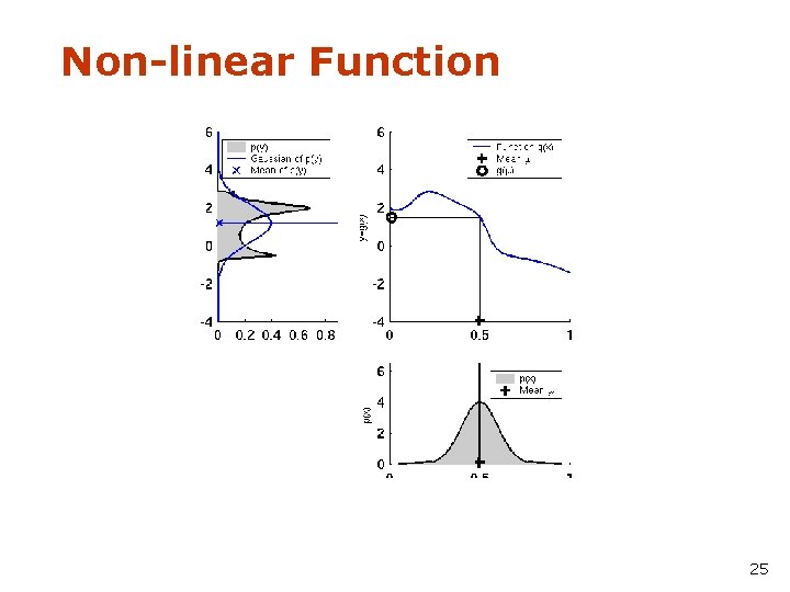
Nonlinear Dynamic Systems • Most realistic robotic problems involve nonlinear functions 23

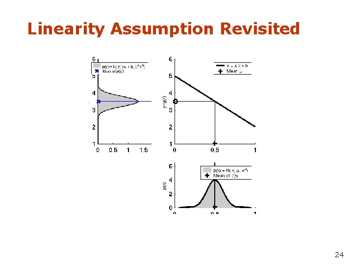
Linearity Assumption Revisited 24

Non-linear Function 25

EKF Linearization (1) 26

EKF Linearization (2) 27

EKF Linearization (3) 28

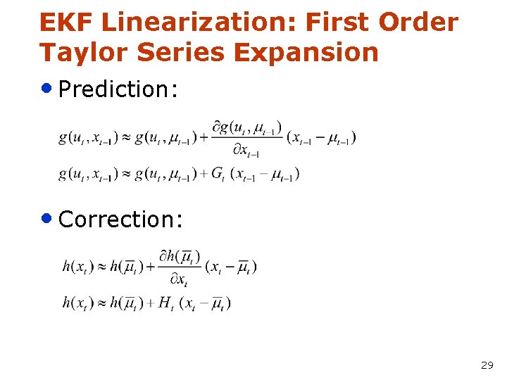
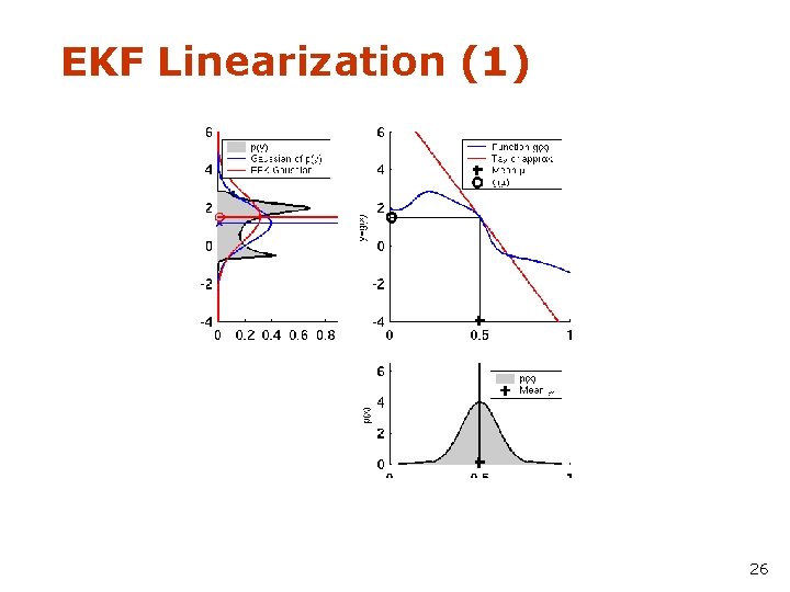
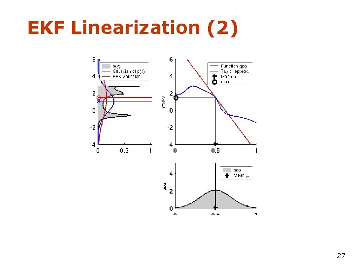
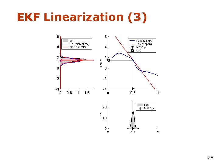
EKF Linearization: First Order Taylor Series Expansion • Prediction: • Correction: 29

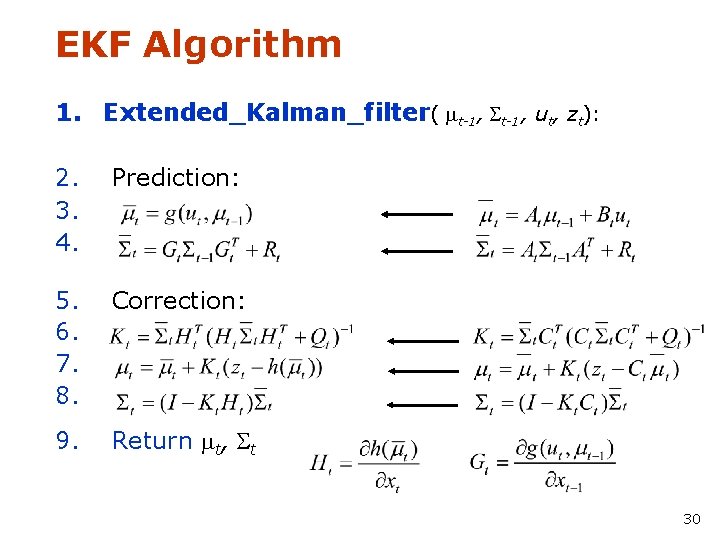
EKF Algorithm 1. Extended_Kalman_filter( mt-1, St-1, ut, zt): 2. 3. 4. Prediction: 5. 6. 7. 8. Correction: 9. Return mt, St 30

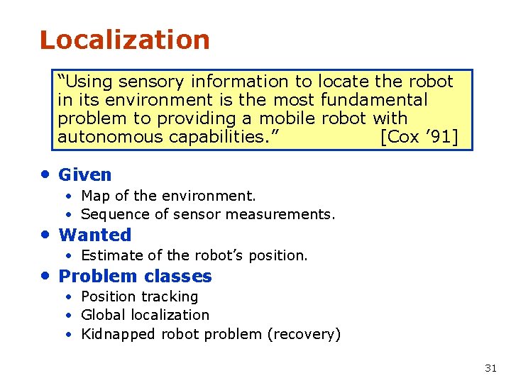
Localization “Using sensory information to locate the robot in its environment is the most fundamental problem to providing a mobile robot with autonomous capabilities. ” [Cox ’ 91] • Given • Map of the environment. • Sequence of sensor measurements. • Wanted • Estimate of the robot’s position. • Problem classes • Position tracking • Global localization • Kidnapped robot problem (recovery) 31

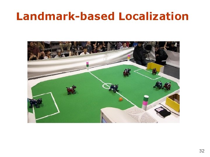
Landmark-based Localization 32

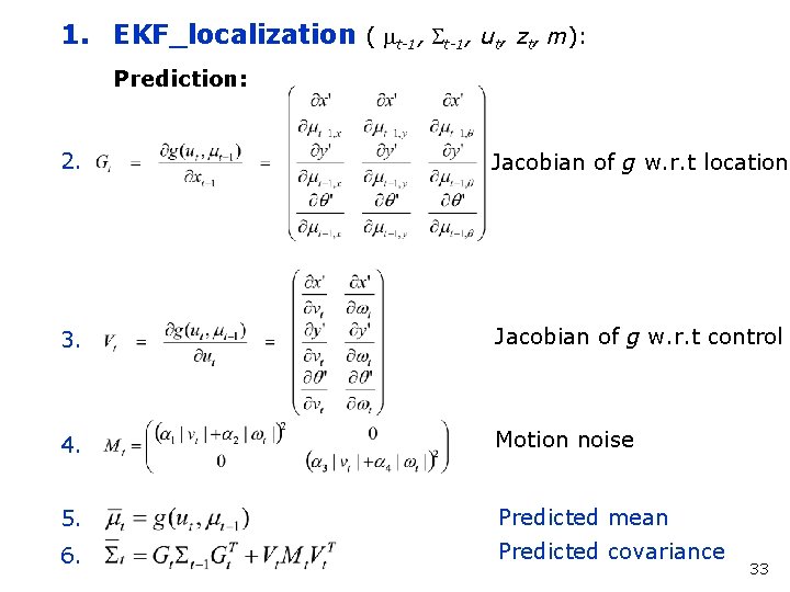
1. EKF_localization ( mt-1, St-1, ut, zt, m): Prediction: 2. Jacobian of g w. r. t location 3. Jacobian of g w. r. t control 4. Motion noise 5. Predicted mean 6. Predicted covariance 33

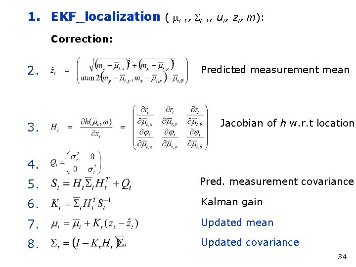
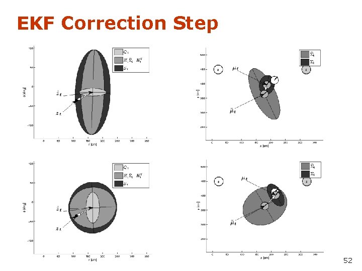
1. EKF_localization ( mt-1, St-1, ut, zt, m): Correction: 2. 3. Predicted measurement mean Jacobian of h w. r. t location 4. 5. Pred. measurement covariance 6. Kalman gain 7. Updated mean 8. Updated covariance 34

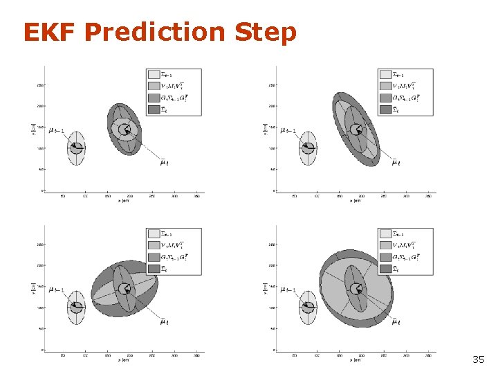
EKF Prediction Step 35

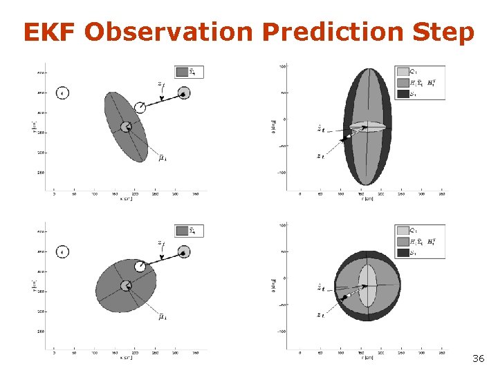
EKF Observation Prediction Step 36

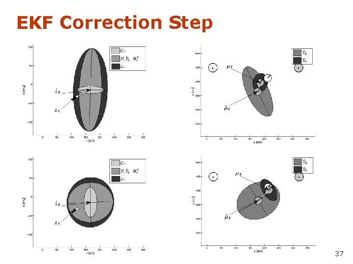
EKF Correction Step 37

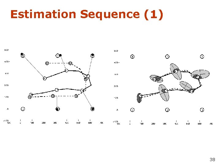
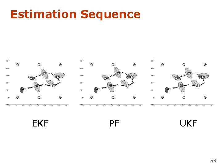
Estimation Sequence (1) 38

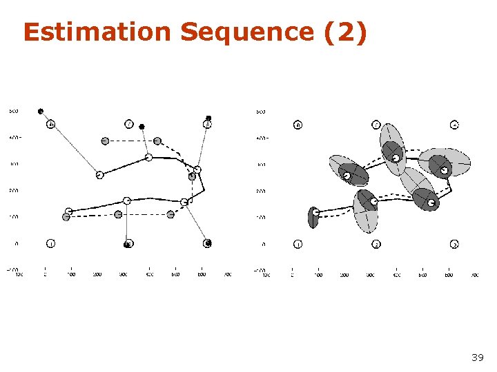
Estimation Sequence (2) 39

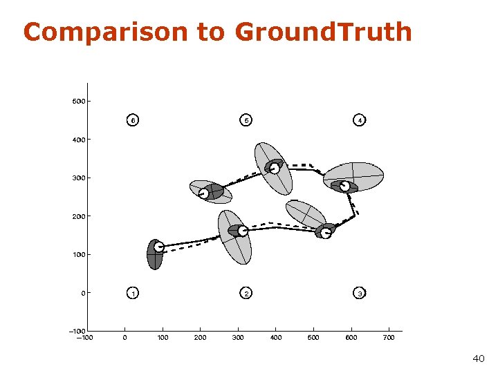
Comparison to Ground. Truth 40

EKF Summary • Highly efficient: Polynomial in measurement dimensionality k and state dimensionality n: O(k 2. 376 + n 2) • Not optimal! • Can diverge if nonlinearities are large! • Works surprisingly well even when all assumptions are violated! 41

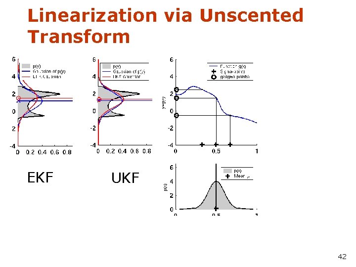
Linearization via Unscented Transform EKF UKF 42

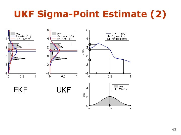
UKF Sigma-Point Estimate (2) EKF UKF 43

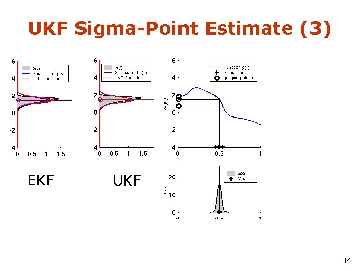
UKF Sigma-Point Estimate (3) EKF UKF 44

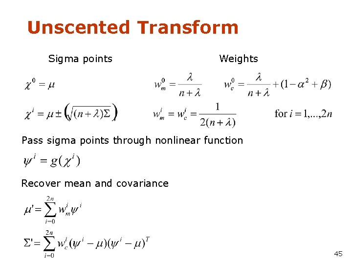
Unscented Transform Sigma points Weights Pass sigma points through nonlinear function Recover mean and covariance 45

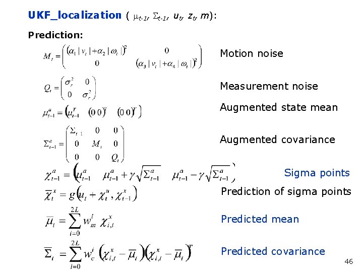
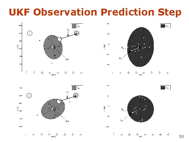
UKF_localization ( mt-1, St-1, ut, zt, m): Prediction: Motion noise Measurement noise Augmented state mean Augmented covariance Sigma points Prediction of sigma points Predicted mean Predicted covariance 46

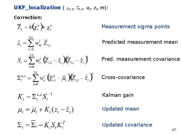
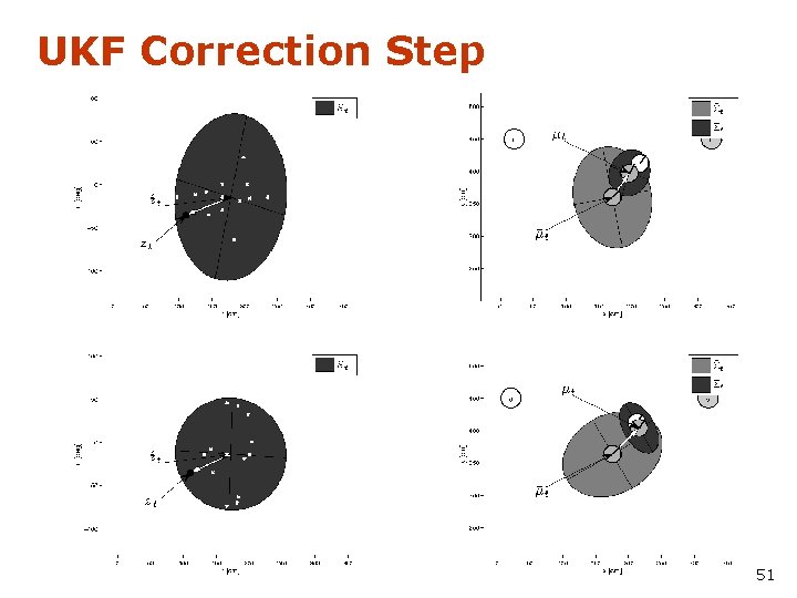
UKF_localization ( mt-1, St-1, ut, zt, m): Correction: Measurement sigma points Predicted measurement mean Pred. measurement covariance Cross-covariance Kalman gain Updated mean Updated covariance 47

1. EKF_localization ( mt-1, St-1, ut, zt, m): Correction: 2. 3. Predicted measurement mean Jacobian of h w. r. t location 4. 5. Pred. measurement covariance 6. Kalman gain 7. Updated mean 8. Updated covariance 48

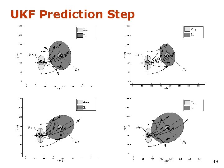
UKF Prediction Step 49

UKF Observation Prediction Step 50

UKF Correction Step 51

EKF Correction Step 52

Estimation Sequence EKF PF UKF 53

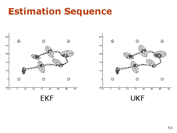
Estimation Sequence EKF UKF 54

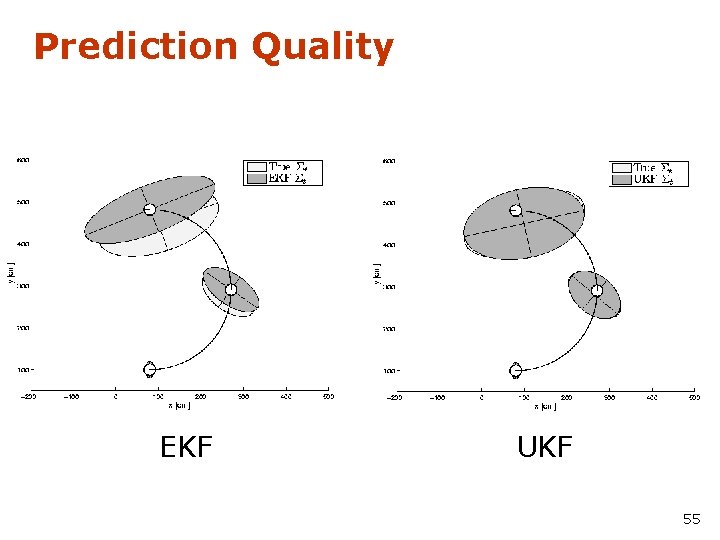
Prediction Quality EKF UKF 55

UKF Summary • Highly efficient: Same complexity as EKF, with a constant factor slower in typical practical applications • Better linearization than EKF: Accurate in first two terms of Taylor expansion (EKF only first term) • Derivative-free: No Jacobians needed • Still not optimal! 56

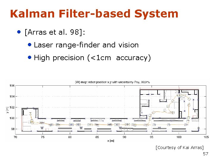
Kalman Filter-based System • [Arras et al. 98]: • Laser range-finder and vision • High precision (<1 cm accuracy) [Courtesy of Kai Arras] 57

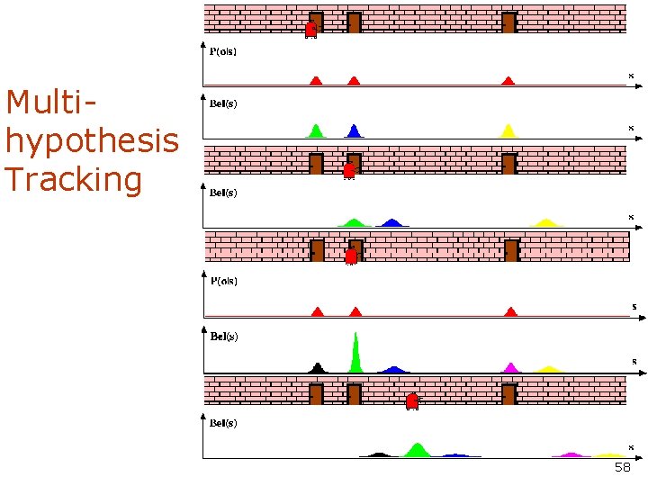
Multihypothesis Tracking 58

Localization With MHT • Belief is represented by multiple hypotheses • Each hypothesis is tracked by a Kalman filter • Additional problems: • Data association: Which observation corresponds to which hypothesis? • Hypothesis management: When to add / delete hypotheses? • Huge body of literature on target tracking, motion correspondence etc. 59

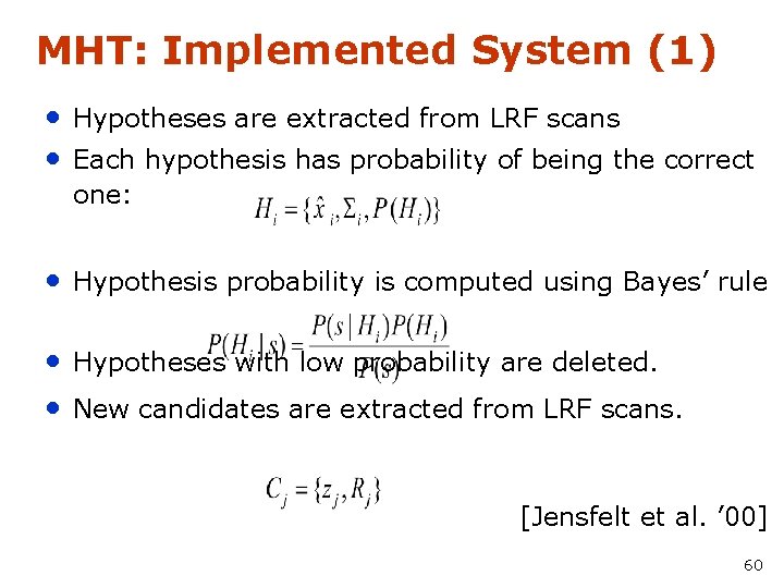
MHT: Implemented System (1) • Hypotheses are extracted from LRF scans • Each hypothesis has probability of being the correct one: • Hypothesis probability is computed using Bayes’ rule • Hypotheses with low probability are deleted. • New candidates are extracted from LRF scans. [Jensfelt et al. ’ 00] 60

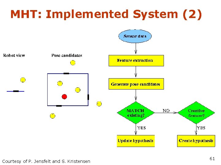
MHT: Implemented System (2) Courtesy of P. Jensfelt and S. Kristensen 61

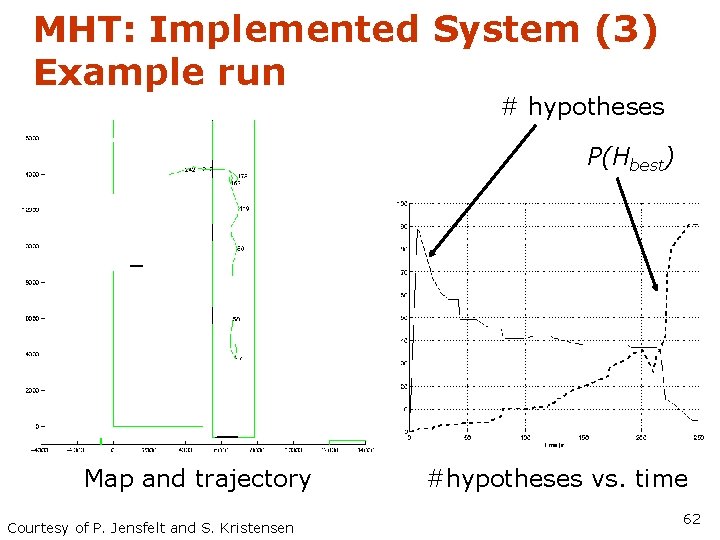
MHT: Implemented System (3) Example run # hypotheses P(Hbest) Map and trajectory Courtesy of P. Jensfelt and S. Kristensen #hypotheses vs. time 62