Slides for Chapter 3 Output knowledge representation of

Slides for Chapter 3, Output: knowledge representation of Data Mining by I. H. Witten, E. Frank, M. A. Hall and C. J. Pal

Output: Knowledge representation • • • Tables Linear models Trees Rules Classification rules Association rules Rules with exceptions More expressive rules Instance-based representation Clusters 2

Output: representing structural patterns • Many different ways of representing patterns • Decision trees, rules, instance-based, … • • Also called “knowledge” representation Representation determines inference method Understanding the output is the key to understanding the underlying learning methods Different types of output for different learning problems (e. g. , classification, regression, …) 3

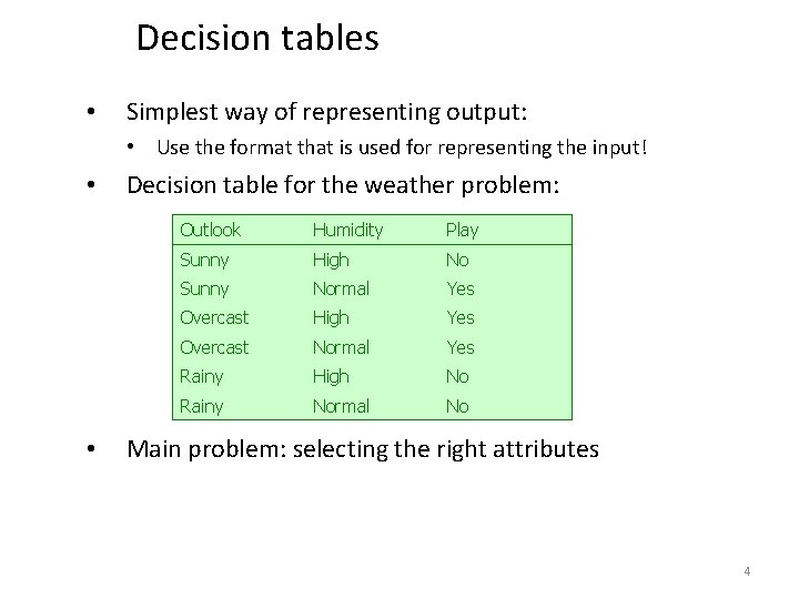
Decision tables • Simplest way of representing output: • Use the format that is used for representing the input! • • Decision table for the weather problem: Outlook Humidity Play Sunny High No Sunny Normal Yes Overcast High Yes Overcast Normal Yes Rainy High No Rainy Normal No Main problem: selecting the right attributes 4

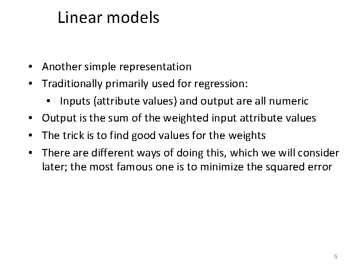
Linear models • Another simple representation • Traditionally primarily used for regression: • Inputs (attribute values) and output are all numeric • Output is the sum of the weighted input attribute values • The trick is to find good values for the weights • There are different ways of doing this, which we will consider later; the most famous one is to minimize the squared error 5

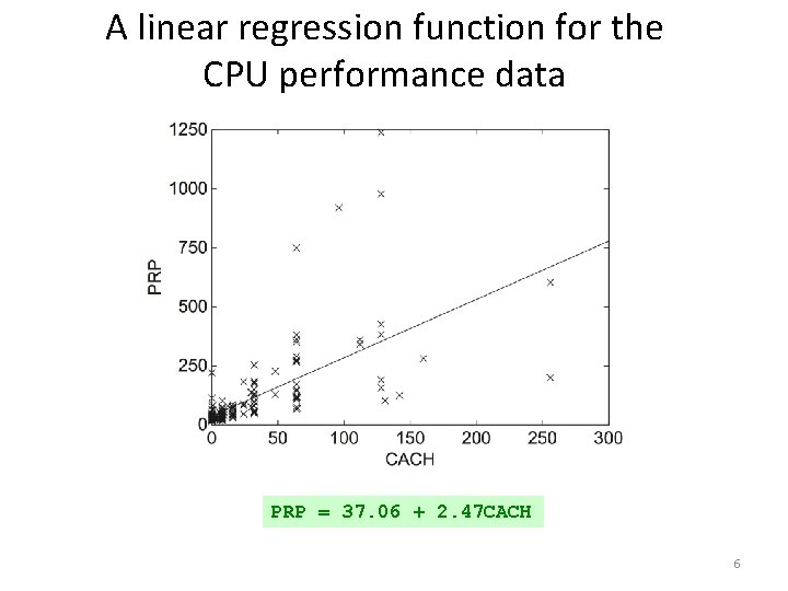
A linear regression function for the CPU performance data PRP = 37. 06 + 2. 47 CACH 6

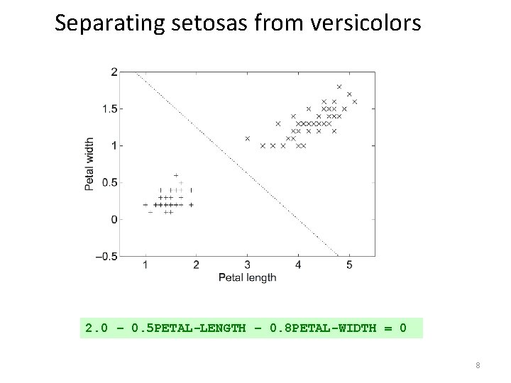
Linear models for classification • Binary classification • Line separates the two classes • Decision boundary - defines where the decision changes from one class value to the other • Prediction is made by plugging in observed values of the attributes into the expression • Predict one class if output 0, and the other class if output < 0 • Boundary becomes a high-dimensional plane (hyperplane) when there are multiple attributes 7

Separating setosas from versicolors 2. 0 – 0. 5 PETAL-LENGTH – 0. 8 PETAL-WIDTH = 0 8

Decision trees • • “Divide-and-conquer” approach produces tree Nodes involve testing a particular attribute Usually, attribute value is compared to constant Other possibilities: • Comparing values of two attributes • Using a function of one or more attributes • Leaves assign classification, set of classifications, or probability distribution to instances • Unknown instance is routed down the tree 9

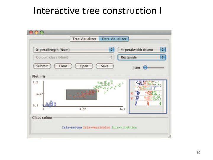
Interactive tree construction I 10

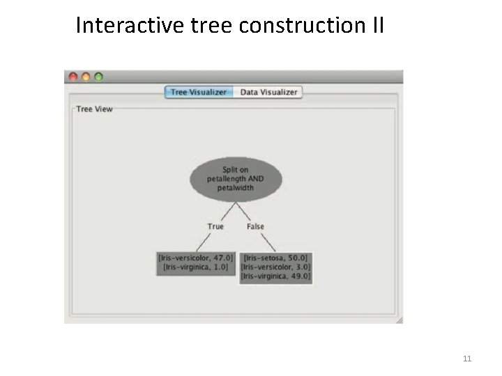
Interactive tree construction II 11

Nominal and numeric attributes in trees • Nominal: number of children usually equal to number values attribute won’t get tested more than once • Other possibility: division into two subsets • Numeric: test whether value is greater or less than constant attribute may get tested several times • Other possibility: three-way split (or multi-way split) • Integer: less than, equal to, greater than • Real: below, within, above 12

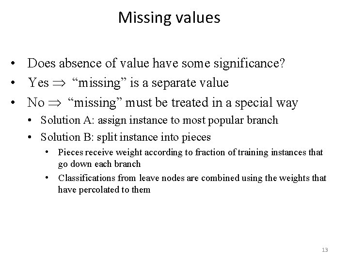
Missing values • Does absence of value have some significance? • Yes “missing” is a separate value • No “missing” must be treated in a special way • Solution A: assign instance to most popular branch • Solution B: split instance into pieces • Pieces receive weight according to fraction of training instances that go down each branch • Classifications from leave nodes are combined using the weights that have percolated to them 13

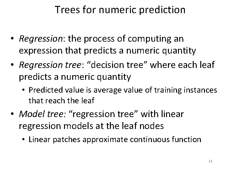
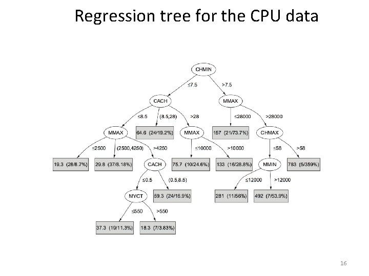
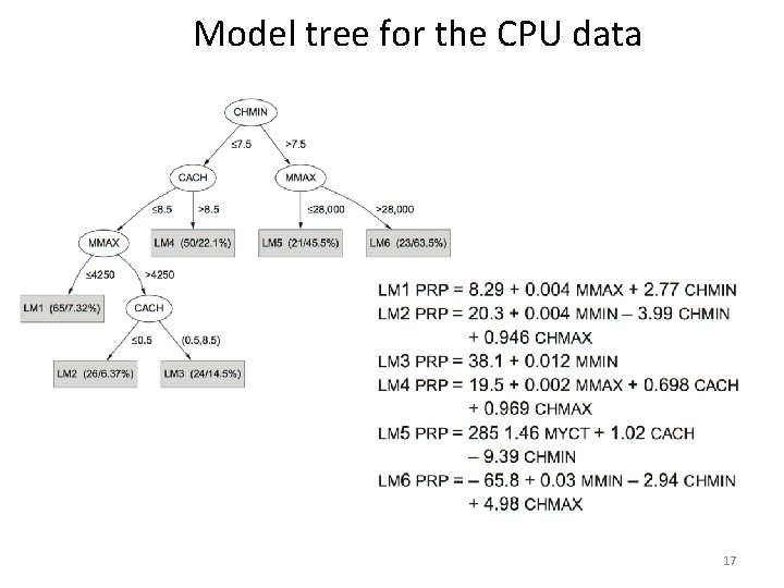
Trees for numeric prediction • Regression: the process of computing an expression that predicts a numeric quantity • Regression tree: “decision tree” where each leaf predicts a numeric quantity • Predicted value is average value of training instances that reach the leaf • Model tree: “regression tree” with linear regression models at the leaf nodes • Linear patches approximate continuous function 14

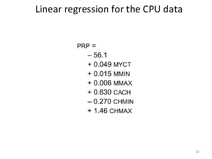
Linear regression for the CPU data PRP = - 56. 1 + 0. 049 MYCT + 0. 015 MMIN + 0. 006 MMAX + 0. 630 CACH - 0. 270 CHMIN + 1. 46 CHMAX 15

Regression tree for the CPU data 16

Model tree for the CPU data 17

Classification rules • • • Popular alternative to decision trees Antecedent (pre-condition): a series of tests (just like the tests at the nodes of a decision tree) Tests are usually logically ANDed together (but may also be general logical expressions) Consequent (conclusion): classes, set of classes, or probability distribution assigned by rule Individual rules are often logically ORed together • Conflicts arise if different conclusions apply 18

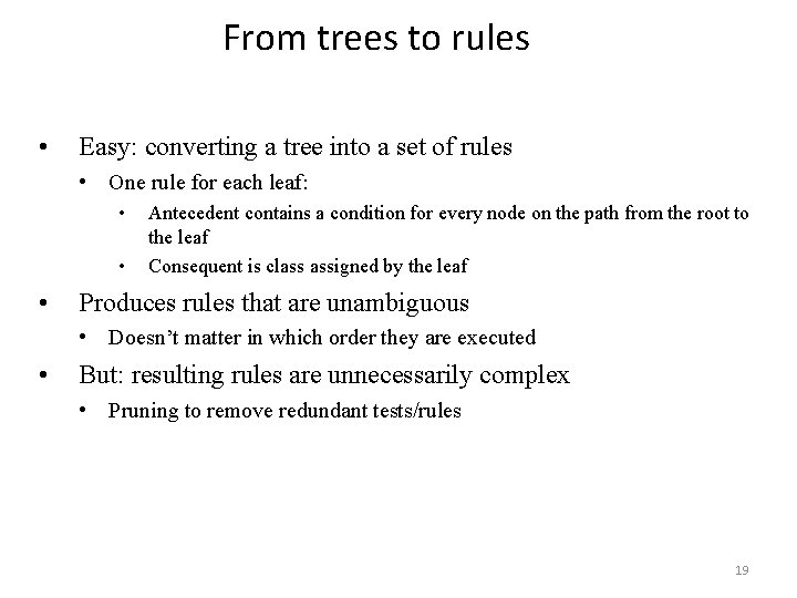
From trees to rules • Easy: converting a tree into a set of rules • One rule for each leaf: • • • Antecedent contains a condition for every node on the path from the root to the leaf Consequent is class assigned by the leaf Produces rules that are unambiguous • Doesn’t matter in which order they are executed • But: resulting rules are unnecessarily complex • Pruning to remove redundant tests/rules 19

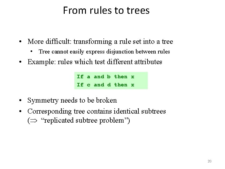
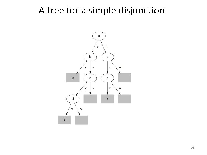
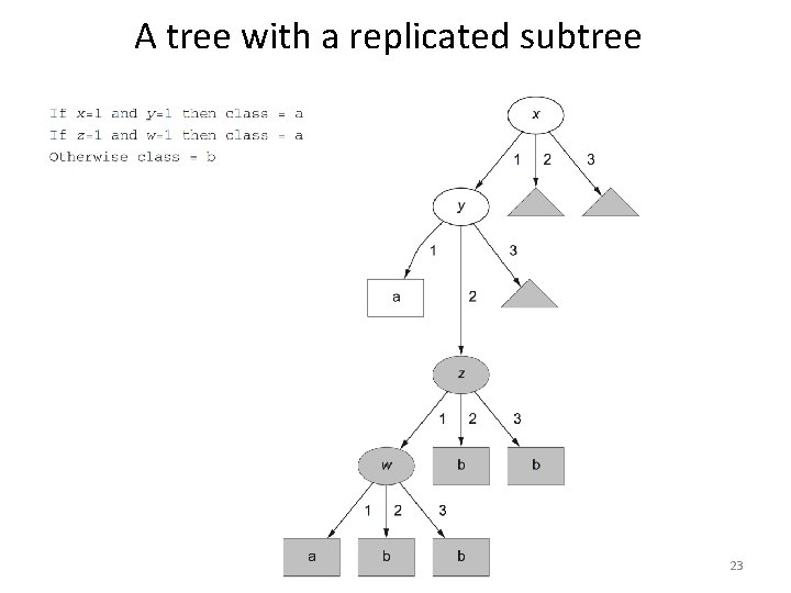
From rules to trees • More difficult: transforming a rule set into a tree • Tree cannot easily express disjunction between rules • Example: rules which test different attributes If a and b then x If c and d then x • Symmetry needs to be broken • Corresponding tree contains identical subtrees ( “replicated subtree problem”) 20

A tree for a simple disjunction 21

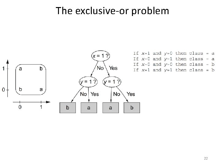
The exclusive-or problem 22

A tree with a replicated subtree 23

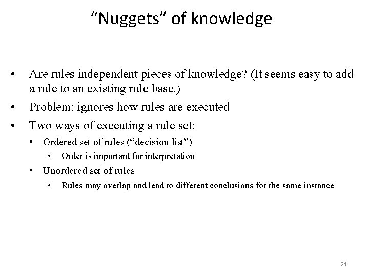
“Nuggets” of knowledge • • • Are rules independent pieces of knowledge? (It seems easy to add a rule to an existing rule base. ) Problem: ignores how rules are executed Two ways of executing a rule set: • Ordered set of rules (“decision list”) • Order is important for interpretation • Unordered set of rules • Rules may overlap and lead to different conclusions for the same instance 24

Interpreting rules • What if two or more rules conflict? • Give no conclusion at all? • Go with rule that is most popular on training data? • … • What if no rule applies to a test instance? • Give no conclusion at all? • Go with class that is most frequent in training data? • … 25

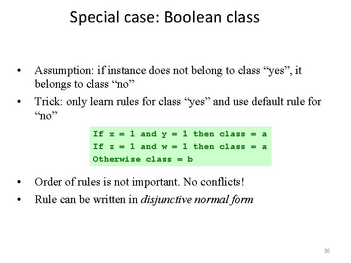
Special case: Boolean class • • Assumption: if instance does not belong to class “yes”, it belongs to class “no” Trick: only learn rules for class “yes” and use default rule for “no” If x = 1 and y = 1 then class = a If z = 1 and w = 1 then class = a Otherwise class = b • • Order of rules is not important. No conflicts! Rule can be written in disjunctive normal form 26

Association rules • Association rules… • … can predict any attribute and combinations of attributes • … are not intended to be used together as a set • Problem: immense number of possible associations • Output needs to be restricted to show only the most predictive associations only those with high support and high confidence 27

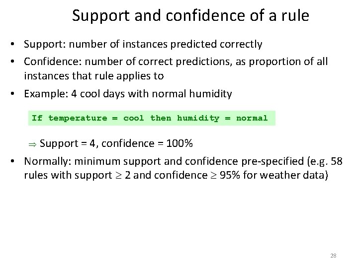
Support and confidence of a rule • Support: number of instances predicted correctly • Confidence: number of correct predictions, as proportion of all instances that rule applies to • Example: 4 cool days with normal humidity If temperature = cool then humidity = normal Support = 4, confidence = 100% • Normally: minimum support and confidence pre-specified (e. g. 58 rules with support 2 and confidence 95% for weather data) 28

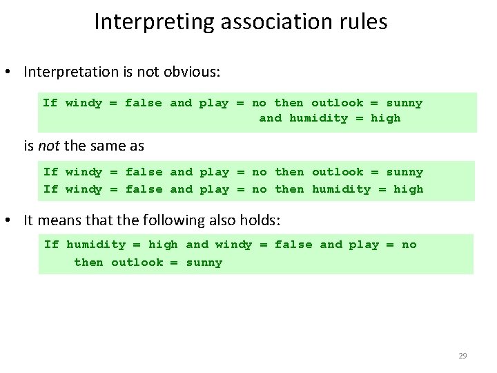
Interpreting association rules • Interpretation is not obvious: If windy = false and play = no then outlook = sunny and humidity = high is not the same as If windy = false and play = no then outlook = sunny If windy = false and play = no then humidity = high • It means that the following also holds: If humidity = high and windy = false and play = no then outlook = sunny 29

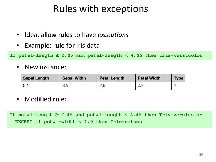
Rules with exceptions • Idea: allow rules to have exceptions • Example: rule for iris data If petal-length 2. 45 and petal-length < 4. 45 then Iris-versicolor • New instance: • Modified rule: If petal-length 2. 45 and petal-length < 4. 45 then Iris-versicolor EXCEPT if petal-width < 1. 0 then Iris-setosa 30

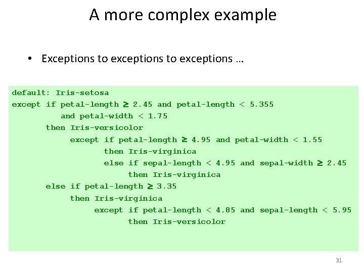
A more complex example • Exceptions to exceptions … default: Iris-setosa except if petal-length 2. 45 and petal-length < 5. 355 and petal-width < 1. 75 then Iris-versicolor except if petal-length 4. 95 and petal-width < 1. 55 then Iris-virginica else if sepal-length < 4. 95 and sepal-width 2. 45 then Iris-virginica else if petal-length 3. 35 then Iris-virginica except if petal-length < 4. 85 and sepal-length < 5. 95 then Iris-versicolor 31

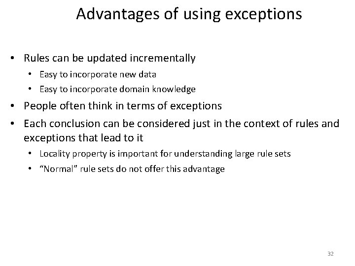
Advantages of using exceptions • Rules can be updated incrementally • Easy to incorporate new data • Easy to incorporate domain knowledge • People often think in terms of exceptions • Each conclusion can be considered just in the context of rules and exceptions that lead to it • Locality property is important for understanding large rule sets • “Normal” rule sets do not offer this advantage 32

More on exceptions • Default. . . except if. . . then. . . is logically equivalent to if. . . then. . . else (where the “else” specifies what the “default” does) • But: exceptions offer a psychological advantage – Assumption: defaults and tests early on apply more widely than exceptions further down – Exceptions reflect special cases 33

Rules involving relations • So far: all rules involved comparing an attribute-value to a constant (e. g. temperature < 45) • These rules are called “propositional” because they have the same expressive power as propositional logic • What if problem involves relationships between examples (e. g. family tree problem from above)? • Can’t be expressed with propositional rules • More expressive representation required 34

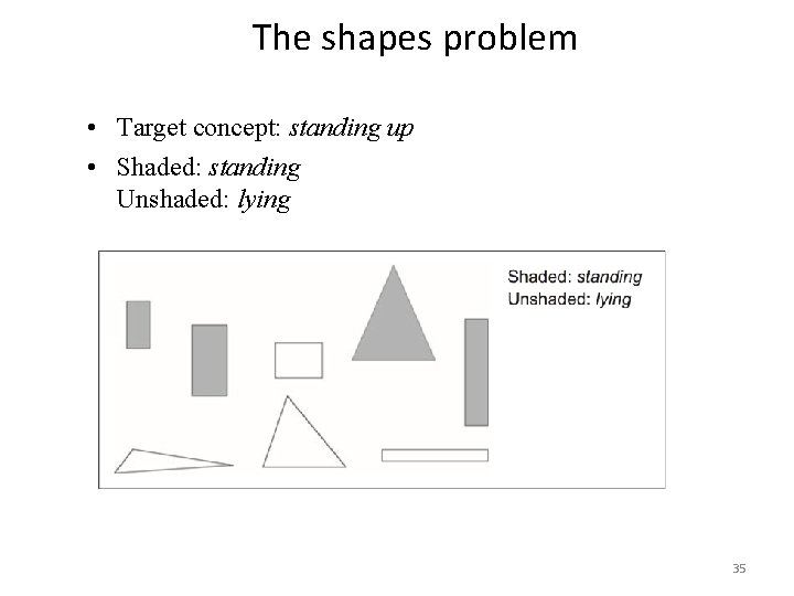
The shapes problem • Target concept: standing up • Shaded: standing Unshaded: lying 35

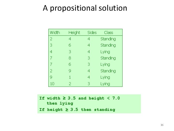
A propositional solution Width Height Sides Class 2 4 4 Standing 3 6 4 Standing 4 3 4 Lying 7 8 3 Standing 7 6 3 Lying 2 9 4 Standing 9 1 4 Lying 10 2 3 Lying If width 3. 5 and height < 7. 0 then lying If height 3. 5 then standing 36

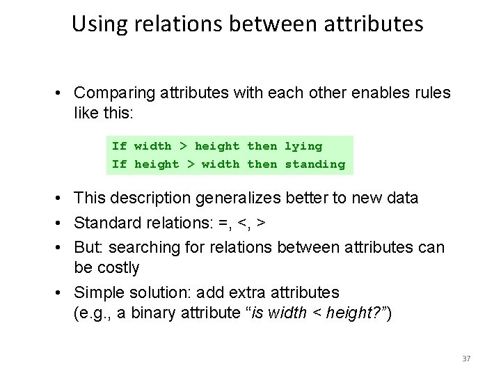
Using relations between attributes • Comparing attributes with each other enables rules like this: If width > height then lying If height > width then standing • This description generalizes better to new data • Standard relations: =, <, > • But: searching for relations between attributes can be costly • Simple solution: add extra attributes (e. g. , a binary attribute “is width < height? ”) 37

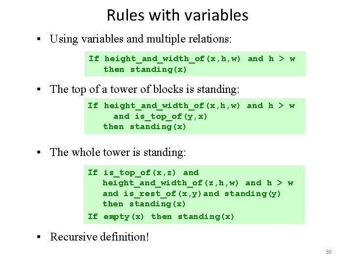
Rules with variables • Using variables and multiple relations: If height_and_width_of(x, h, w) and h > w then standing(x) • The top of a tower of blocks is standing: If height_and_width_of(x, h, w) and h > w and is_top_of(y, x) then standing(x) • The whole tower is standing: If is_top_of(x, z) and height_and_width_of(z, h, w) and h > w and is_rest_of(x, y)and standing(y) then standing(x) If empty(x) then standing(x) • Recursive definition! 38

Inductive logic programming • Recursive definition can be seen as logic program • Techniques for learning logic programs stem from the area of “inductive logic programming” (ILP) • But: recursive definitions are hard to learn • Also: few practical problems require recursion • Thus: many ILP techniques are restricted to non-recursive definitions to make learning easier 39

Instance-based representation • Simplest form of learning: rote learning • Training instances are searched for instance that most closely resembles new instance • The instances themselves represent the knowledge • Also called instance-based learning • Similarity function defines what’s “learned” • Instance-based learning is lazy learning • Methods: nearest-neighbor, k-nearest-neighbor, … 40

The distance function • Simplest case: one numeric attribute • Distance is the difference between the two attribute values involved (or a function thereof) • Several numeric attributes: normally, Euclidean distance is used and attributes are normalized • Nominal attributes: distance is set to 1 if values are different, 0 if they are equal • Are all attributes equally important? • Weighting the attributes might be necessary 41

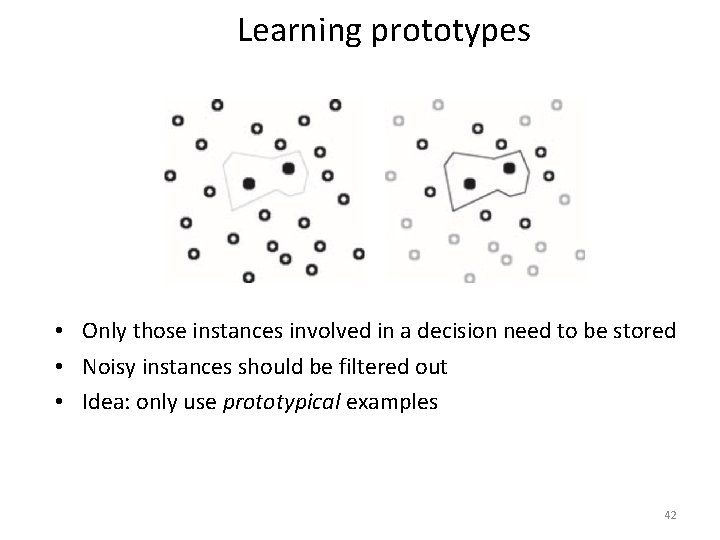
Learning prototypes • Only those instances involved in a decision need to be stored • Noisy instances should be filtered out • Idea: only use prototypical examples 42

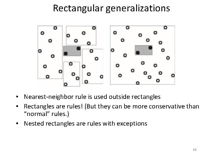
Rectangular generalizations • Nearest-neighbor rule is used outside rectangles • Rectangles are rules! (But they can be more conservative than “normal” rules. ) • Nested rectangles are rules with exceptions 43

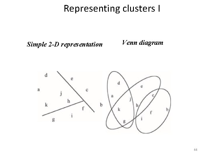
Representing clusters I Simple 2 -D representation Venn diagram 44

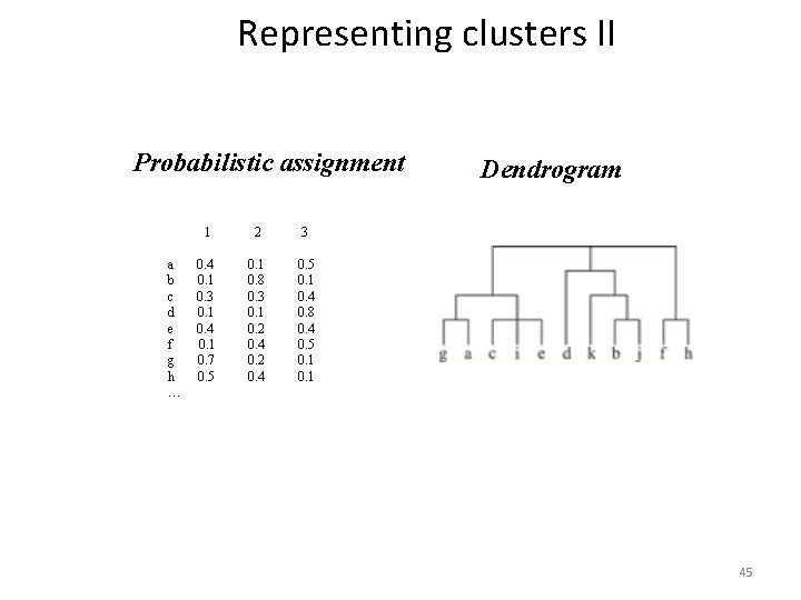
Representing clusters II Probabilistic assignment a b c d e f g h … 1 2 3 0. 4 0. 1 0. 3 0. 1 0. 4 0. 1 0. 7 0. 5 0. 1 0. 8 0. 3 0. 1 0. 2 0. 4 0. 5 0. 1 0. 4 0. 8 0. 4 0. 5 0. 1 Dendrogram NB: dendron is the Greek word for tree 45