SLIDES BY Yaochen Kuo KAINAN University Slide 1

. . SLIDES. BY. . Yaochen Kuo. . KAINAN. . University. Slide 1
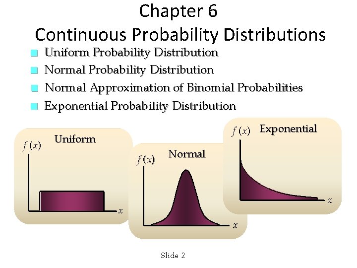
Chapter 6 Continuous Probability Distributions n n f (x) Uniform Probability Distribution Normal Approximation of Binomial Probabilities Exponential Probability Distribution f (x) Exponential Uniform f (x ) Normal x x x Slide 2
Continuous Probability Distributions n A continuous random variable can assume any value in an interval on the real line or in a collection of intervals. n It is not possible to talk about the probability of the random variable assuming a particular value. n Instead, we talk about the probability of the random variable assuming a value within a given interval. Slide 3
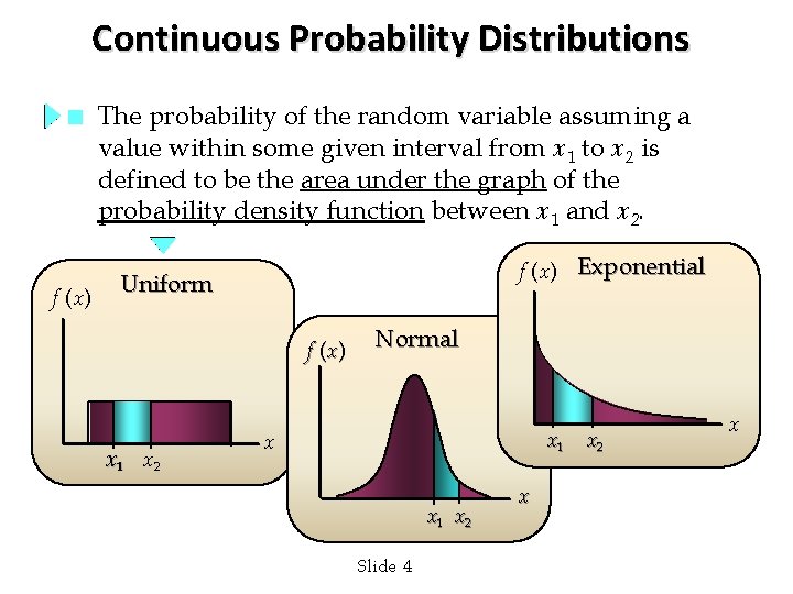
Continuous Probability Distributions n f (x) The probability of the random variable assuming a value within some given interval from x 1 to x 2 is defined to be the area under the graph of the probability density function between x 1 and x 2. f (x) Exponential Uniform f (x ) x 1 x 2 Normal x 1 xx 12 x x 1 x 2 Slide 4 x x

Uniform Probability Distribution n A random variable is uniformly distributed whenever the probability is proportional to the interval’s length. n The uniform probability density function is: f (x) = 1/(b – a) for a < x < b =0 elsewhere: a = smallest value the variable can assume b = largest value the variable can assume Slide 5
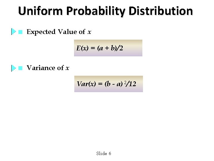
Uniform Probability Distribution n Expected Value of x E(x) = (a + b)/2 n Variance of x Var(x) = (b - a) 2/12 Slide 6
Uniform Probability Distribution n Example: The flight time of an airplane Consider the random variable x representing the flight time of an airplane traveling from Chicago to New York. Suppose the flight time can be any value in the interval from 120 minutes to 140 minutes. Let’s assume that sufficient actual flight data are available to conclude that the probability of a flight time within any 1 -minute interval is the same as the probability of a flight time within any other 1 -minute interval contained in the larger interval from 120 to 140 minutes. Slide 7

Uniform Probability Distribution n Uniform Probability Density Function f(x) = 1/20 for 120 < x < 140 =0 elsewhere: x = the flight time of an airplane traveling from Chicago to New York Slide 8
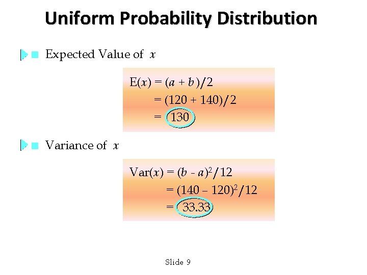
Uniform Probability Distribution n Expected Value of x E(x) = (a + b)/2 = (120 + 140)/2 = 130 n Variance of x Var(x) = (b - a)2/12 = (140 – 120)2/12 = 33. 33 Slide 9
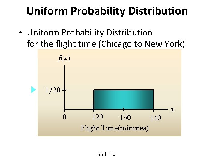
Uniform Probability Distribution • Uniform Probability Distribution for the flight time (Chicago to New York) f(x) 1/20 0 120 130 140 Flight Time(minutes) Slide 10 x
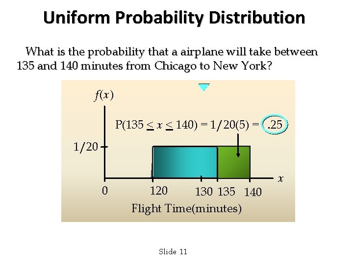
Uniform Probability Distribution What is the probability that a airplane will take between 135 and 140 minutes from Chicago to New York? f(x) P(135 < x < 140) = 1/20(5) =. 25 1/20 0 120 135 140 Flight Time(minutes) Slide 11 x
Area as a Measure of Probability n n n The area under the graph of f (x) and probability are identical. This is valid for all continuous random variables. The probability that x takes on a value between some lower value x 1 and some higher value x 2 can be found by computing the area under the graph of f (x) over the interval from x 1 to x 2. Slide 12
Normal Probability Distribution n The normal probability distribution is the most important distribution for describing a continuous random variable. It is widely used in statistical inference. It has been used in a wide variety of applications including: • Heights of people • Rainfall amounts • Test scores • Scientific measurements Slide 13
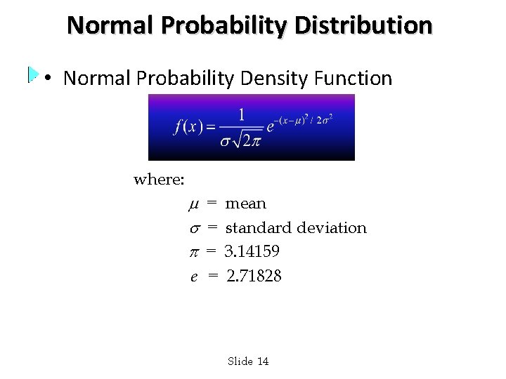
Normal Probability Distribution • Normal Probability Density Function where: = mean = standard deviation = 3. 14159 e = 2. 71828 Slide 14
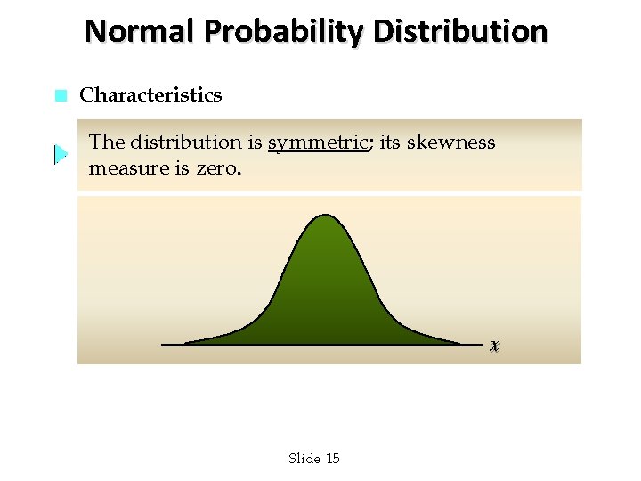
Normal Probability Distribution n Characteristics The distribution is symmetric; its skewness measure is zero. x Slide 15
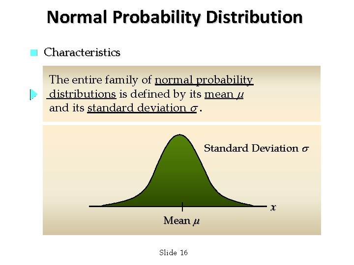
Normal Probability Distribution n Characteristics The entire family of normal probability distributions is defined by its mean and its standard deviation . Standard Deviation Mean Slide 16 x
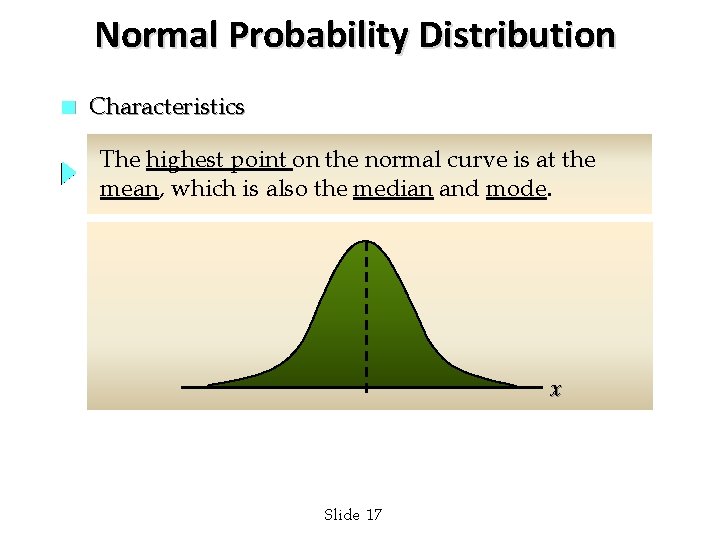
Normal Probability Distribution n Characteristics The highest point on the normal curve is at the mean, which is also the median and mode. x Slide 17
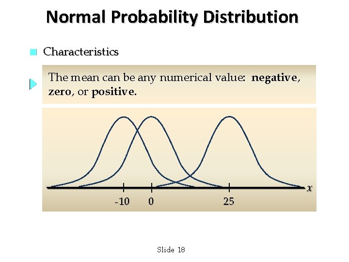
Normal Probability Distribution n Characteristics The mean can be any numerical value: negative, zero, or positive. -10 0 25 Slide 18 x
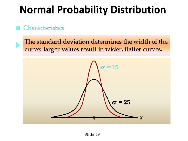
Normal Probability Distribution n Characteristics The standard deviation determines the width of the curve: larger values result in wider, flatter curves. s = 15 s = 25 x Slide 19
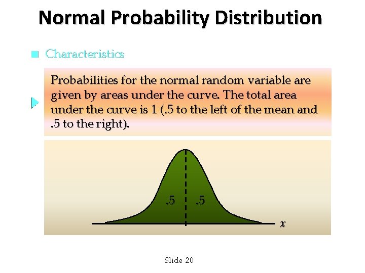
Normal Probability Distribution n Characteristics Probabilities for the normal random variable are given by areas under the curve. The total area under the curve is 1 (. 5 to the left of the mean and. 5 to the right). . 5 x Slide 20
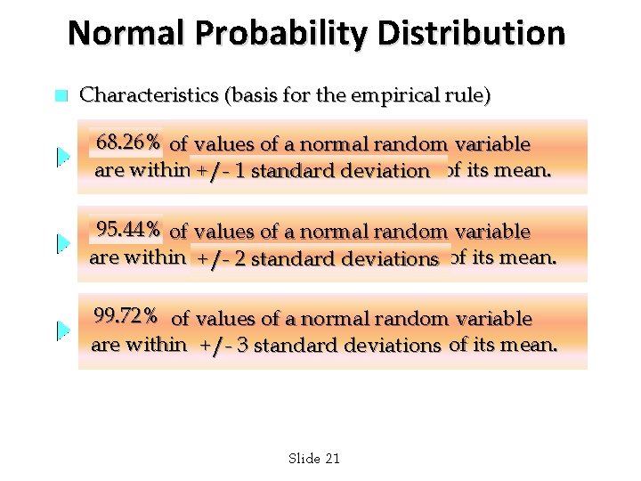
Normal Probability Distribution n Characteristics (basis for the empirical rule) 68. 26% of values of a normal random variable are within +/- 1 standard deviation of its mean. 95. 44% of values of a normal random variable are within +/- 2 standard deviations of its mean. 99. 72% of values of a normal random variable are within +/- 3 standard deviations of its mean. Slide 21
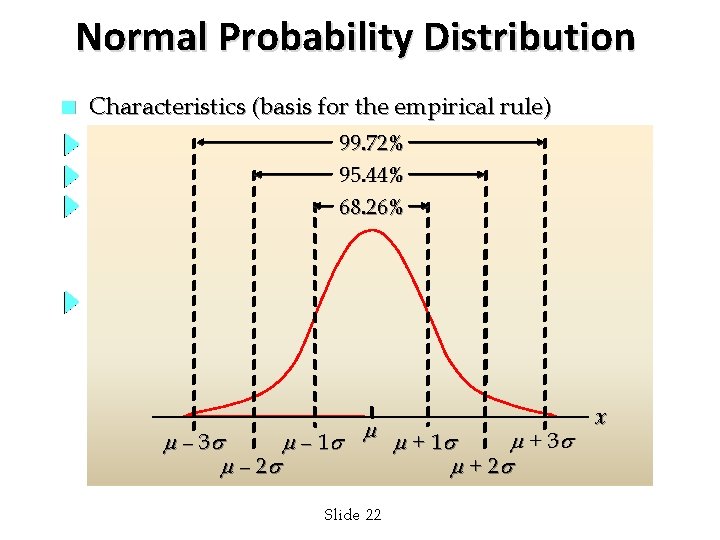
Normal Probability Distribution n Characteristics (basis for the empirical rule) 99. 72% 95. 44% 68. 26% + 3 – 1 + 1 – 2 + 2 Slide 22 x
Standard Normal Probability Distribution n Characteristics A random variable having a normal distribution with a mean of 0 and a standard deviation of 1 is said to have a standard normal probability distribution. Slide 23
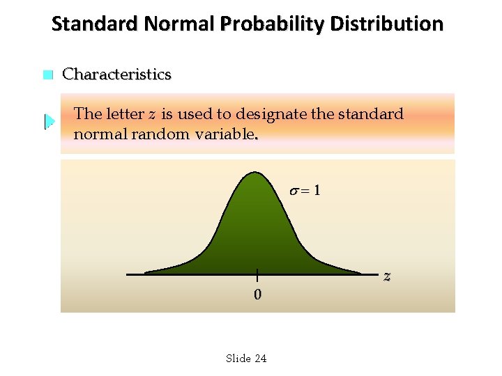
Standard Normal Probability Distribution n Characteristics The letter z is used to designate the standard normal random variable. = 1 0 Slide 24 z
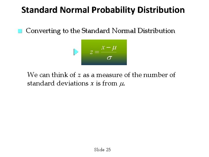
Standard Normal Probability Distribution n Converting to the Standard Normal Distribution We can think of z as a measure of the number of standard deviations x is from . Slide 25
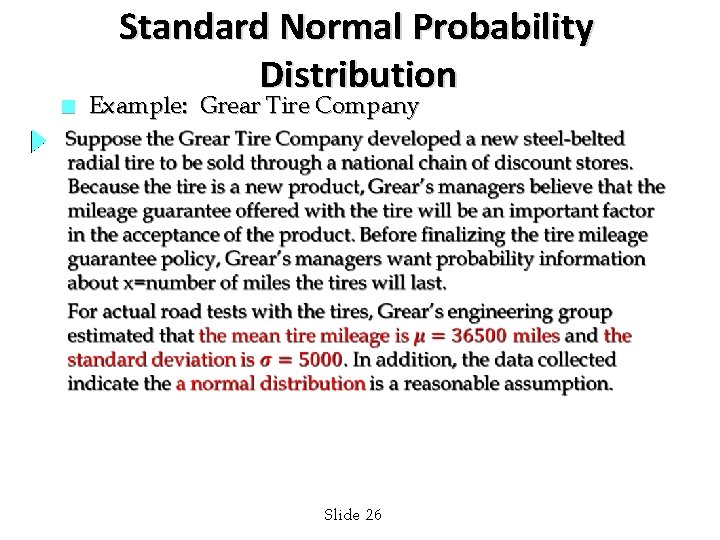
n Standard Normal Probability Distribution Example: Grear Tire Company Slide 26
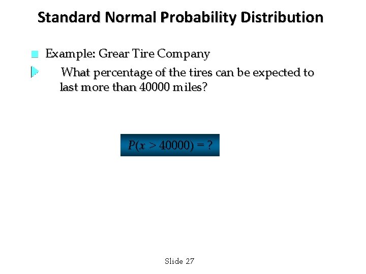
Standard Normal Probability Distribution n Example: Grear Tire Company What percentage of the tires can be expected to last more than 40000 miles? P(x > 40000) = ? Slide 27
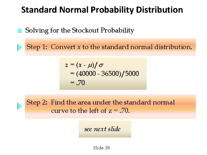
Standard Normal Probability Distribution n Solving for the Stockout Probability Step 1: Convert x to the standard normal distribution. z = (x - )/ = (40000 - 36500)/5000 =. 70 Step 2: Find the area under the standard normal curve to the left of z =. 70. see next slide Slide 28
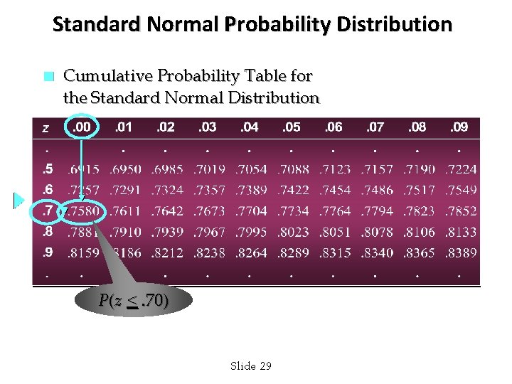
Standard Normal Probability Distribution n Cumulative Probability Table for the Standard Normal Distribution P(z <. 70) Slide 29
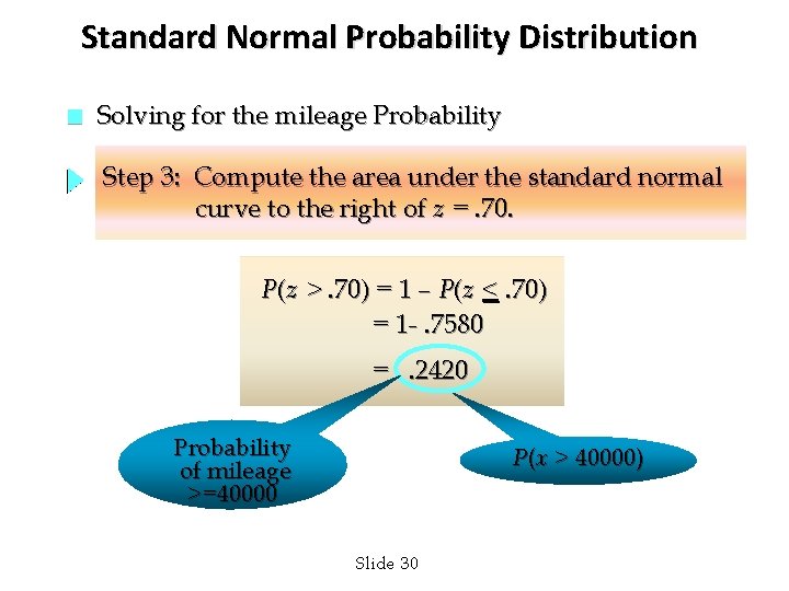
Standard Normal Probability Distribution n Solving for the mileage Probability Step 3: Compute the area under the standard normal curve to the right of z =. 70. P(z >. 70) = 1 – P(z <. 70) = 1 -. 7580 =. 2420 Probability of mileage >=40000 P(x > 40000) Slide 30
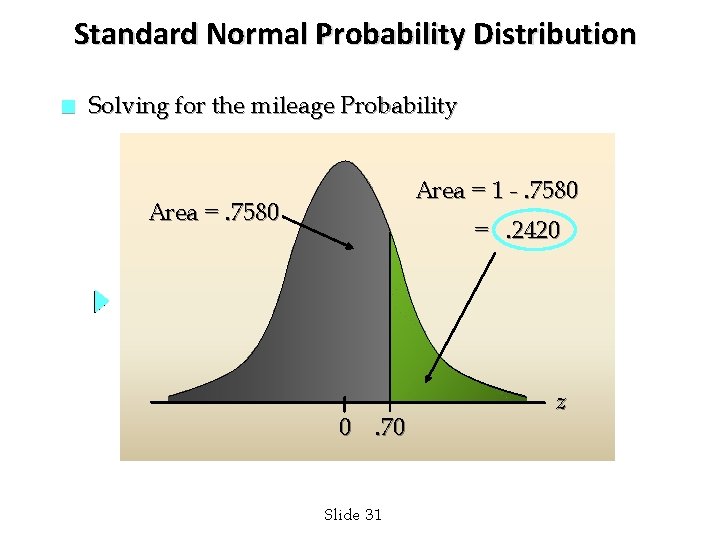
Standard Normal Probability Distribution n Solving for the mileage Probability Area = 1 -. 7580 Area =. 7580 =. 2420 0. 70 Slide 31 z
Standard Normal Probability Distribution • Standard Normal Probability Distribution Let us assume that Grear is considering a guarantee that will provide a discount on replacement tires if the original tires do not provide the guaranteed mileage. What should the guarantee mileage be if Grear wants no more than 10% of the tires to be eligible for the discount guarantee? Slide 32
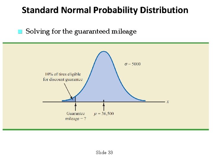
Standard Normal Probability Distribution n Solving for the guaranteed mileage Slide 33
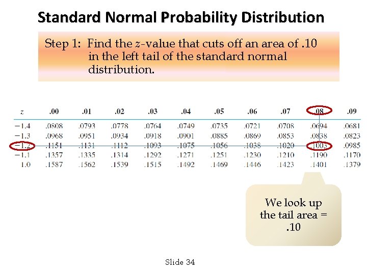
Standard Normal Probability Distribution Step 1: Find the z-value that cuts off an area of. 10 in the left tail of the standard normal distribution. We look up the tail area =. 10 Slide 34
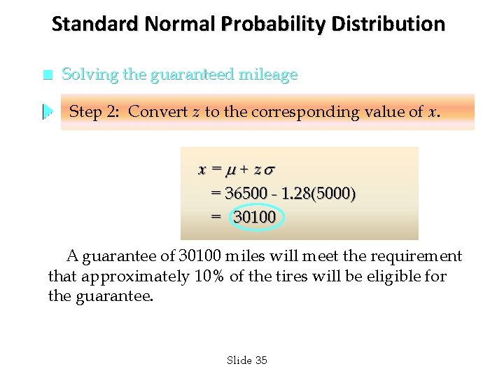
Standard Normal Probability Distribution n Solving the guaranteed mileage Step 2: Convert z to the corresponding value of x. x = + z = 36500 - 1. 28(5000) = 30100 A guarantee of 30100 miles will meet the requirement that approximately 10% of the tires will be eligible for the guarantee. Slide 35
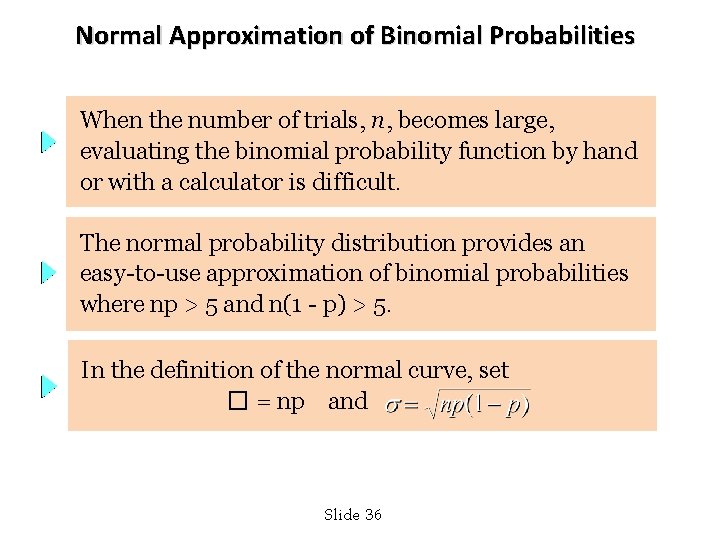
Normal Approximation of Binomial Probabilities When the number of trials, n, becomes large, evaluating the binomial probability function by hand or with a calculator is difficult. The normal probability distribution provides an easy-to-use approximation of binomial probabilities where np > 5 and n(1 - p) > 5. In the definition of the normal curve, set � = np and Slide 36
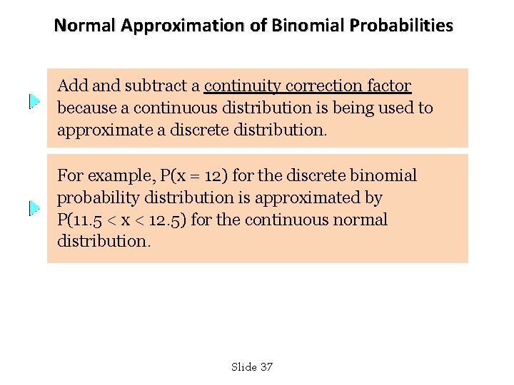
Normal Approximation of Binomial Probabilities Add and subtract a continuity correction factor because a continuous distribution is being used to approximate a discrete distribution. For example, P(x = 12) for the discrete binomial probability distribution is approximated by P(11. 5 < x < 12. 5) for the continuous normal distribution. Slide 37
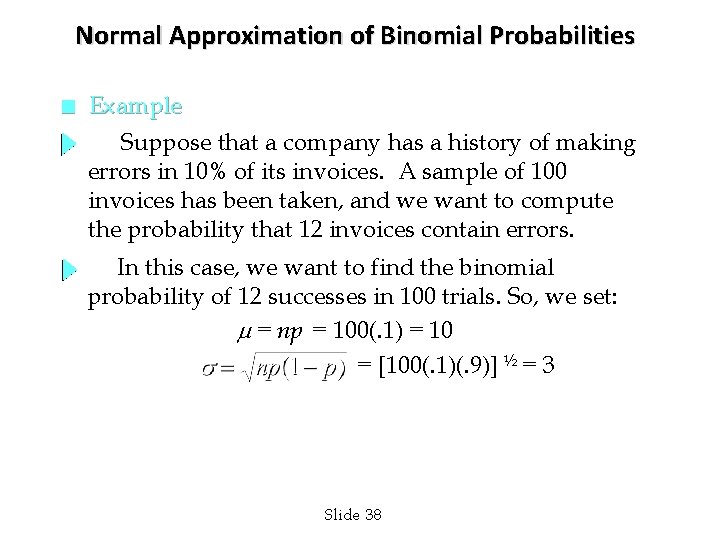
Normal Approximation of Binomial Probabilities n Example Suppose that a company has a history of making errors in 10% of its invoices. A sample of 100 invoices has been taken, and we want to compute the probability that 12 invoices contain errors. In this case, we want to find the binomial probability of 12 successes in 100 trials. So, we set: = np = 100(. 1) = 10 = [100(. 1)(. 9)] ½ = 3 Slide 38
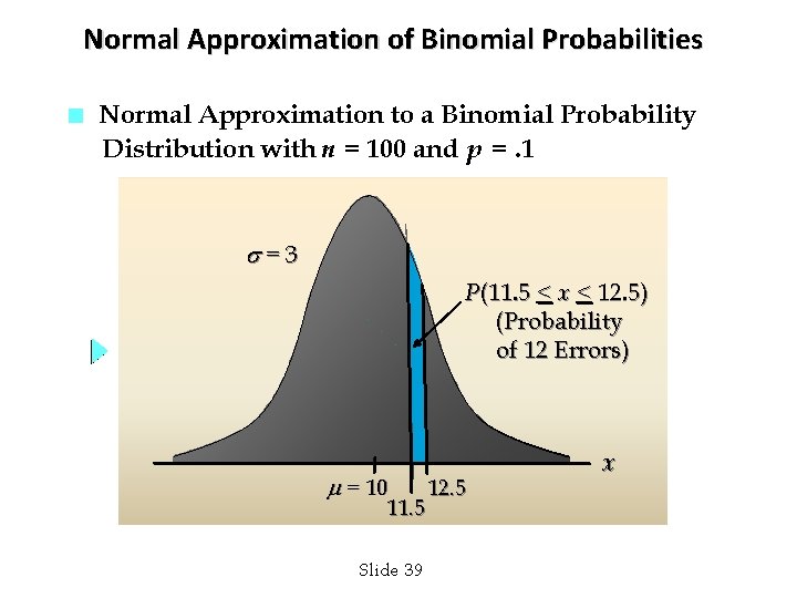
Normal Approximation of Binomial Probabilities n Normal Approximation to a Binomial Probability Distribution with n = 100 and p =. 1 =3 P(11. 5 < x < 12. 5) (Probability of 12 Errors) = 10 11. 5 Slide 39 12. 5 x
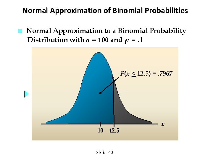
Normal Approximation of Binomial Probabilities n Normal Approximation to a Binomial Probability Distribution with n = 100 and p =. 1 P(x < 12. 5) =. 7967 10 12. 5 Slide 40 x
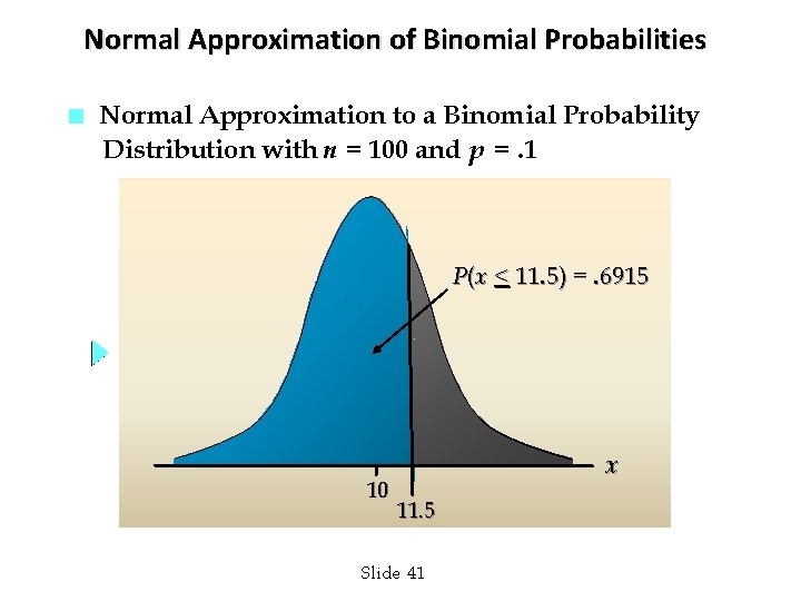
Normal Approximation of Binomial Probabilities n Normal Approximation to a Binomial Probability Distribution with n = 100 and p =. 1 P(x < 11. 5) =. 6915 10 x 11. 5 Slide 41
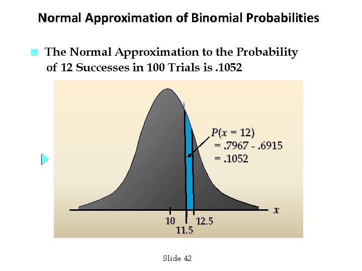
Normal Approximation of Binomial Probabilities n The Normal Approximation to the Probability of 12 Successes in 100 Trials is. 1052 P(x = 12) =. 7967 -. 6915 =. 1052 10 12. 5 11. 5 Slide 42 x
Exponential Probability Distribution n The exponential probability distribution is useful in describing the time it takes to complete a task. The exponential random variables can be used to describe: • Time between vehicle arrivals at a toll booth • Time required to complete a questionnaire • Distance between major defects in a highway In waiting line applications, the exponential distribution is often used for service times. Slide 43
Exponential Probability Distribution n A property of the exponential distribution is that the mean and standard deviation are equal. n The exponential distribution is skewed to the right. Its skewness measure is 2. Slide 44
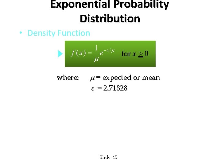
Exponential Probability Distribution • Density Function for x > 0 where: = expected or mean e = 2. 71828 Slide 45
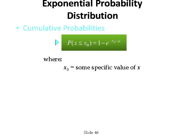
Exponential Probability Distribution • Cumulative Probabilities where: x 0 = some specific value of x Slide 46
Exponential Probability Distribution n Example: Al’s Full-Service Pump The time between arrivals of cars at Al’s fullservice gas pump follows an exponential probability distribution with a mean time between arrivals of 3 minutes. Al would like to know the probability that the time between two successive arrivals will be 2 minutes or less. Slide 47
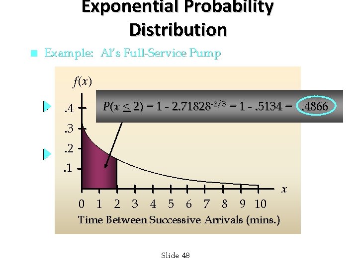
Exponential Probability Distribution n Example: Al’s Full-Service Pump f(x) P(x < 2) = 1 - 2. 71828 -2/3 = 1 -. 5134 =. 4866 . 4. 3. 2. 1 x 0 1 2 3 4 5 6 7 8 9 10 Time Between Successive Arrivals (mins. ) Slide 48
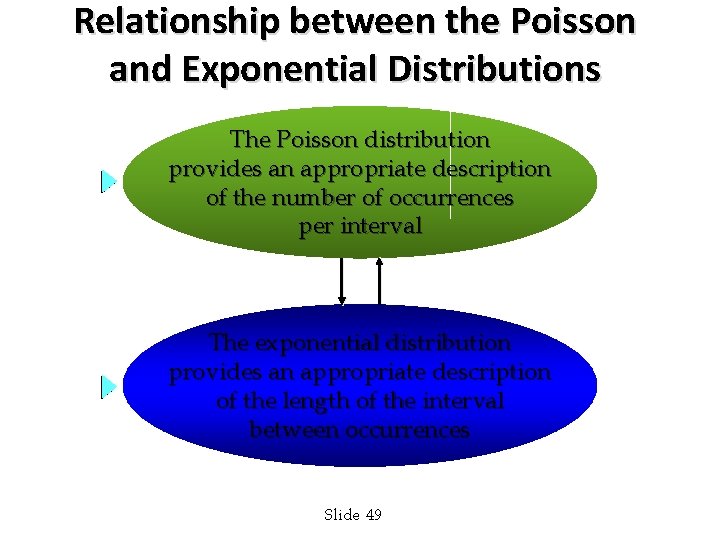
Relationship between the Poisson and Exponential Distributions The Poisson distribution provides an appropriate description of the number of occurrences per interval The exponential distribution provides an appropriate description of the length of the interval between occurrences Slide 49

End of Chapter 6 Slide 50
- Slides: 50