Slides available http www comp nus edu sgxiangnanpapersicf

Slides available: http: //www. comp. nus. edu. sg/~xiangnan/papers/icf. pptx Collaborative Filtering for Implicit Feedback Dr. He Xiangnan (何向南) School of Computing National University of Singapore December 2016 1

Outline • Background • Work #1 (shallow model): – He et al. SIGIR 2016: Fast Matrix Factorization for Online Recommendation with Implicit Feedback • Work #2 (deep model): – He et al. WWW 2017: Neural Collaborative Filtering. http: //www. comp. nus. edu. sg/~xiangnan/papers/ncf. pdf 2

Value of Recommender System (RS) • Netflix: 60+% of the movies watched are recommended. • Google News: RS generates 38% more click-through • Amazon: 35% sales from recommendations Statistics come from Xavier Amatriain 3

Collaborative Filtering (CF) “CF makes predictions (filtering) about a user’s interest by collecting preferences information from many users (collaborating)” 1. Neighbor-based: - Do prediction based on the similarity of users/items. 2. Model-based: - Assume data is generated by an underlying model. 4

Matrix Factorization (MF) • MF is the most popular model-based CF technique: – Linear latent factor model: User 'u' rated an item 'i' Learn latent vector for each user, item: Affinity between user ‘u’ and item ‘i’: 5

MF on Explicit Feedback • Explicit feedback, e. g. users’ ratings on movies, where a user explicitly indicates whether he/she likes an item or not. • Well-formed problem – both users’ positive & negative feedback are available. Model: Objective Function (regression): Only observed ratings are considered! 6

But for Implicit Feedback… • Implicit feedback, e. g. , users’ clicks/watches/purchases on items, where a user implicitly expresses his/her preference. users User 'u' rated an item 'i’, but we do not know whether he likes it 1 0 0 1 Due to the prevalence or not!! of implicit feedback, 0 1 0 0 recent on RS has shifted to implicit 1 1 0 research 0 - More like a classification problem, 1 0 0 1 feedback! rather than regression. 0/1 Interaction matrix - Unobserved data (0 entries) are crucial to consider! 7

Challenges for Learning from Implicit Feedback 1 0 0 1 1 0 0 1 0/1 Interaction matrix 1. The full user-item matrix need to be considered. - # of training instance: M ✕ N; - Unrealistic to deal with real-world data. 2. An ill-formed problem: - No true-negative preference data; - 0 entries are a mixture of negative and unknown feedback. 8

Previous Implicit MF Solutions Pair-wise Ranking Method (BPR, Rendle et al, UAI 2009) Sampling negative instances: LIKELIHOOD: All Items not bought by u Sigmoid: Regression-based Method (WALS, Hu et al, ICDM 2008) Treating all missing data as negative: LOSS: Weight for Missing data Prediction for Prediction on Work #1: Address both missing data observed entries the effectiveness and efficiency Pros: offull regression method. + issue Model the data (good recall) Pros: + Efficient + Optimized for ranking (good precision) Cons: - Less efficient - Only model partial data (low recall) - Uniform weighting on missing data. 9

Work #1: SIGIR 2016. Fast Matrix Factorization for Online Recommendation with Implicit Feedback. Drawbacks of Existing Methods (whole-data based) 10

Drawback #1: Uniform Weighting - Limits model’s fidelity and flexibility • Uniform weighting on missing data assumes that “all missing entries are equally likely to be a negative assessment. ” – The design choice is for the optimization efficiency --- an efficient ALS algorithm (Hu, ICDM 2008) can be derived with uniform weighting. • However, such an assumption is unrealistic. – Item popularity is typically non-uniformly distributed. – Popular items are more likely to be known by users. Tag: ECML'09 Challenge Selection Frequency BBC Video Rank Figures adopt from Rendle, WSDM 2014. Tag Rank 11

Drawback #2: Low Efficiency - Difficult for large-scale data • An analytical solution known as ridge regression – Vector-wise ALS – Time complexity: O((M+N)K 3 + MNK 2) Scary complexity and unrealistic for practical usage M: # of items, N: # of users, K: # of latent factors • With the uniform weighting, Hu can reduce the complexity to O((M+N)K 3 + |R|K 2) |R| denotes the number of observed entries. • However, the complexity is too high for large dataset: – K can be thousands for sufficient model expressiveness e. g. You. Tube RS, which has over billions of users and videos. 12

Drawback #3: - Difficult to support online learning • Scenario of Recommender System: Historical data New data Training Recommendation Time • New data continuously streams in: – New users; – Old users have new interactions; • It is extremely useful to provide instant personalization for new users, and refresh recommendation for old users, but retraining the full model is expensive => Online Incremental Learning 13

Key Features Our method: - Non-uniform weighting on Missing data - An efficient learning algorithm (K times faster than Hu’s ALS, the same magnitude with BPR-SGD learner) - Seamlessly support online learning. 14

#1. Item-Oriented Weighting on Missing Data Old Design: Our Proposal: The confidence that item i missed by users is a true negative assessment Popularity-aware Weighting Scheme: - Similar to frequency-aware negative sampling in word 2 vec. Intuition: a popular item is more likely to be known by users, thus a missing on it is more probably that the user is not interested with it. Overall weight of missing data Frequency of item Smoothness: 0. 5 works well 15

#2. Optimization (Coordinate Descent) • Existing algorithms do not work: – SGD: needs to scan all training instance O(MN). – ALS: requires a uniform weight on missing data. • We develop a Coordinate Descent learner to optimize the whole -data based MF: – Element-wise Alternating Least Squares Learner (e. ALS) – Optimize one latent factor with others fixed (greedy exact optimization) Property e. ALS (ours) ALS (traditional) Optimization Unit Latent factor Latent vector Matrix Inversion No Yes (ridge regression) Time Complexity O(MNK) O((M+N)K 3 + MNK 2) 16

#2. 1 Efficient e. ALS Learner • An efficient learner by using memoization. • Key idea: memoizing the computation for missing data part: Bottleneck: Missing data part • Reformulating the loss function: Sum over all user-item pairs, can be seen as a prior over all interactions! This term can be computed efficiently in O(|R| + MK 2), rather than O(MNK). Algorithm details see our paper. 17

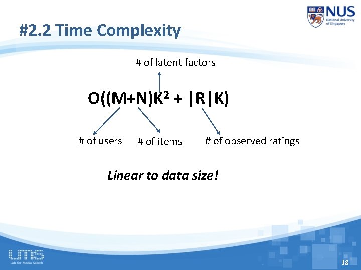
#2. 2 Time Complexity # of latent factors O((M+N)K 2 + |R|K) # of users # of items # of observed ratings Linear to data size! 18

#3. Online Incremental Learning Users Items Given a new (u, i) interaction, how to refresh model parameters without retraining the full model? Our solution: only perform updates for vu and vi Black: old training data Blue: new incoming data - We think the new interaction should change the local features for u and i significantly; While the global picture remains largely unchanged. Pros: + Localized complexity: O(K 2 + (|Ru| + |Ri|)K) 19

Outline • Background • Work #1 (shallow model): – Existing Work – Method – Experiments • Offline Evaluation • Online Evaluation • Work #2 (deep model): – He et al. WWW 2017. Neural Collaborative Filtering. 20

Dataset & Baselines • Two public datasets (filtered at threshold 10): – Yelp Challenge (Dec 2015, ~1. 6 Million reviews) – Amazon Movies (SNAP. Stanford) Dataset Interaction# Item# User# Sparsity Yelp 731, 671 25. 8 K 25. 7 K 99. 89% Amazon 5, 020, 705 75. 3 K 117. 2 K 99. 94% • Baselines: – ALS (Hu et al, ICDM’ 08) – RCD (Devooght et al, KDD’ 15) Randomized Coordinate Descent, state-of-the-art implicit MF solution. – BPR (Rendle et al, UAI’ 09) SGD learner, Pair-wise ranking with sampled missing data. 21

Offline Protocol (Static data) • Leave-one-out evaluation (Rendle et al, UAI’ 09) – Hold out the latest interaction for each user as test (ground-truth). • Although it is widely used in literatures, it is an artificial split that does not reflect the real scenario. – Leak of collaborative information! – New users problem is averted. • Top-K Recommendation (K=100): – Rank all items for a user (very time consuming, longer than training!) – Measure: Hit Ratio and NDCG. – Parameters: #factors = 128 (others are also fairly tuned, see the paper) 22

Compare whole-data based MF e. ALS > ALS: popularity-aware weighting on missing data is useful. 23

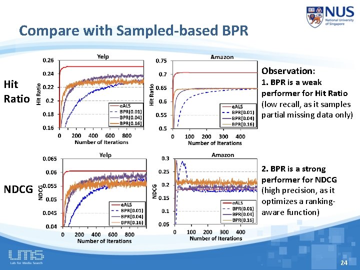
Compare with Sampled-based BPR Hit Ratio NDCG Observation: 1. BPR is a weak performer for Hit Ratio (low recall, as it samples partial missing data only) 2. BPR is a strong performer for NDCG (high precision, as it optimizes a rankingaware function) 24

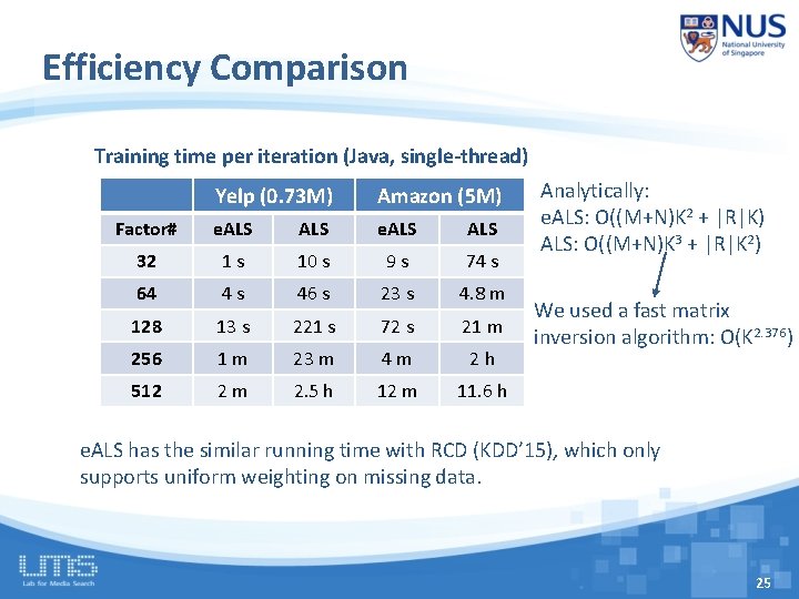
Efficiency Comparison Training time per iteration (Java, single-thread) Yelp (0. 73 M) Amazon (5 M) Factor# e. ALS ALS 32 1 s 10 s 9 s 74 s 64 4 s 46 s 23 s 4. 8 m 128 13 s 221 s 72 s 21 m 256 1 m 23 m 4 m 2 h 512 2 m 2. 5 h 12 m 11. 6 h Analytically: e. ALS: O((M+N)K 2 + |R|K) ALS: O((M+N)K 3 + |R|K 2) We used a fast matrix inversion algorithm: O(K 2. 376) e. ALS has the similar running time with RCD (KDD’ 15), which only supports uniform weighting on missing data. 25

Online Protocol (dynamic data stream) • Sort all interactions by time – Global split at 90%, testing on the latest 10%. Historical data (offline) Training (90%) New Interactions (online) Evaluate & Update Time • In the testing phase: – Given a test interaction (i. e. , u-i pair), the model recommends a Top-K list to evaluate the performance. – Then, the test interaction is fed into the model for an incremental update. • New users problem is obvious: – 57% (Amazon) and 14% (Yelp) test interactions are from new users! 26

Number of Online Iterations Impact of online iterations on e. ALS: Offline training One iteration is enough for e. ALS to converge! While BPR (SGD) needs 5 -10 iterations. 27

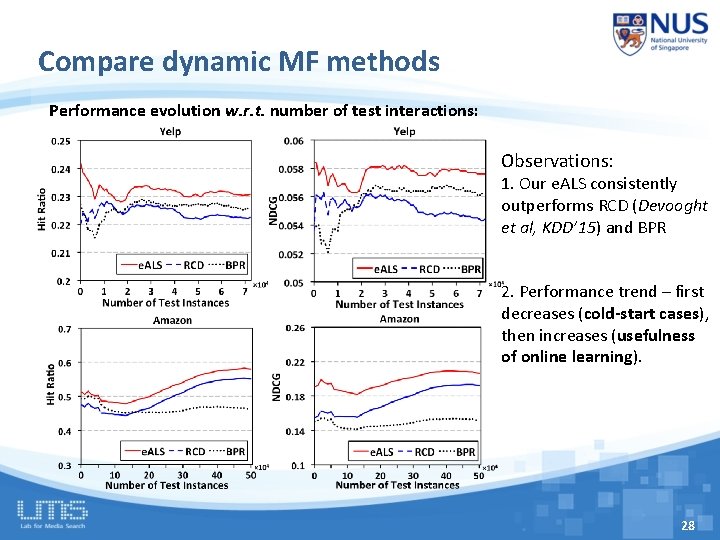
Compare dynamic MF methods Performance evolution w. r. t. number of test interactions: Observations: 1. Our e. ALS consistently outperforms RCD (Devooght et al, KDD’ 15) and BPR 2. Performance trend – first decreases (cold-start cases), then increases (usefulness of online learning). 28

Conclusion of Work #1 • Matrix Factorization for Implicit Feedback – Model the full missing data leads to better prediction recall. – Weight the missing data non-uniformly is more effective. – Develop an efficient algorithm that supports both fast offline training and online learning. • Explore a new way to evaluate recommendation in a more realistic, better manner. – Simulate the dynamic data stream. • Our algorithm has been deployed by a startup company (Rechao 热巢) in streaming news recommendation. 29

Outline • Background • Work #1 (shallow model): – He et al. SIGIR 2016: Fast Matrix Factorization for Online Recommendation with Implicit Feedback • Work #2 (deep model): – He et al. WWW 2017. Neural Collaborative Filtering http: //www. comp. nus. edu. sg/~xiangnan/papers/ncf. pdf) – Motivation – Method – Experiments 30

Limitation of Matrix Factorization • The simple choice of inner product function can limit the expressiveness of a MF model. (E. g. , assuming a unit length) S 42 > S 43 (X) u 1 S 42 > S 43 (X) • Example: sim(u 1, u 2) = 0. 5 sim(u 3, u 1) = 0. 4 sim(u 3, u 2) = 0. 66 u 2 u 3 sim(u 4, u 1) = 0. 6 ***** sim(u 4, u 2) = 0. 2 * sim(u 4, u 3) = 0. 4 *** Jaccard Similarity: 31

Limitation of Matrix Factorization • The simple choice of inner product function can limit the expressiveness of a MF model. assuming a unit length) The inner product can incur a large (E. g. , ranking loss for MF S 42 > S 43 (X) • Example: How to address? u 1 S > S 43 (X) 42 - Using a large number of latent factors; however, it may hurt the u 2) = 0. 5 generalization of the modelsim(u 1, (e. g. overfitting) u 2 sim(u 3, u 1) = 0. 4 Learningsim(u 3, the interaction u 2) = 0. 66 Our solution: function from u 3 data! Rather than the simple, fixed product. sim(u 4, u 1) =inner 0. 6 ***** sim(u 4, u 2) = 0. 2 sim(u 4, u 3) = 0. 4 * *** Jaccard Similarity: 32

Key of this Work Interaction function MF: Inner Product Ours: Learn from Data! 33

Related Work Our work Recommender Deep Learning Systems 34

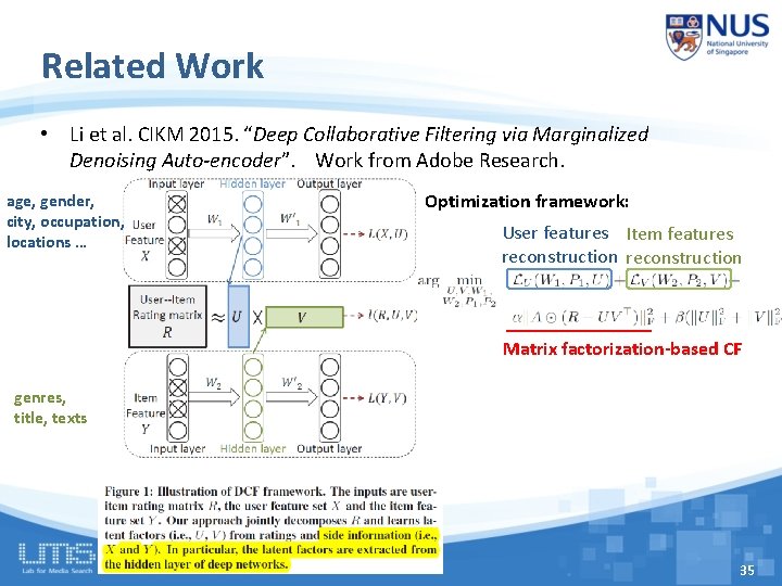
Related Work • Li et al. CIKM 2015. “Deep Collaborative Filtering via Marginalized Denoising Auto-encoder”. Work from Adobe Research. age, gender, city, occupation, locations … Optimization framework: User features Item features reconstruction Matrix factorization-based CF genres, title, texts 35

Related Work • Zhang et al. KDD 2016. “Collaborative Knowledge Base Embedding for Recommender Systems”. Work from Microsoft Research. Inner Product 36

Summarize Related Work • Deep Learning (e. g. , SDAE, CNN, SCAE) is only used for modelling SIDE INFORMATION of users and items. • For modelling the interaction between users and items, existing work still uses the simple inner product (as used in the basic MF). • Other work in a similar vein: – Y. Song et al. SIGIR 2016. "Multi-Rate Deep Learning for Temporal Recommendation“ – H. Wang et al. KDD 2015. "Collaborative deep learning for recommender systems“ – A. Elkahky et al. WWW 2015. "A Multi-View Deep Learning Approach for Cross Domain User Modeling in Recommendation Systems“ – X. Wang et al. MM 2014. "Improving content-based and hybrid music recommendation using deep learning" – Oord et al. NIPS 2013. "Deep content-based music recommendation" 37

Proposed Methods • Our Proposals: – A Neural Collaborative Filtering (NCF) framework that learns the interaction function with a deep neural network. – A NCF instance that generalizes the MF model (GMF). – A NCF instance that models nonlinearities with a multi-layer perceptron (MLP) – A NCF instance Neu. MF that fuses GMF and MLP. 38

NCF Framework NCF uses a multi-layer model to learn the user-item interaction function - Input: sparse feature vector for user u (vu) and item i (vi) - Output: predicted score ŷui Note: Input feature vector can be more than just user/item ID; it can include any categorical variables, such as attributes, contexts and content. 39

Generalized Matrix Factorization (GMF) • NCF can express and generalize MF: Let we define Layer 1 as an element-wise product, and Output Layer as a fully connected layer without bias, we have: 40

Multi-Layer Perceptron (MLP) • NCF can endow more nonlinearities to learn the interaction function: Activation function: Re. LU > tanh > sigmoid Layer 1: Remaining Layers: 41

MF vs. MLP • MF uses an inner product as the interaction function: – Latent factors are independent with each other; – It empirically has good generalization ability for CF modelling (best single model of Netflix and many other recommender tasks). • MLP uses nonlinear functions to learn the interaction function: – Latent factors are not independent with each other; – The interaction function is learnt from data, which theoretically has a better representation ability. – However, its generalization ability is unknown and it is seldom explored in recommender literature/challenge. 42

MF vs. MLP • MF uses an inner product as the interaction function: – Latent factors are independent with each other; – It empirically has good generalization ability for CF modelling (best single model of Netflix and many other recommender tasks). Can we fuse two models to get a more model? – Latent factors are notpowerful independent with each other; • MLP uses a nonlinear function as the interaction function: – The interaction function is learnt from data, which theoretically has a better representation ability. – However, its generalization ability is unknown and it is seldom explored in recommender literature/challenge. 43

44

An Intuitive Solution – Neural Tensor Network • MF model: • MLP model (1 linear layer): • The Neural Tensor Network* naturally assumes MF and MLP share the same embeddings, and combines the outputs of their interaction functions by an addition: • However, we find NTN does not significantly improve over MF: – A possible reason is due to the limitation of the shared embeddings. * Socher Richard, et al. NIPS 2013 "Reasoning with neural tensor networks for knowledge base completion"

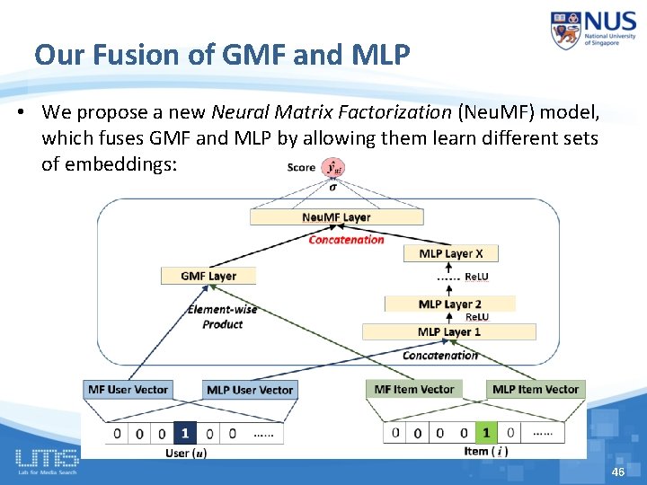
Our Fusion of GMF and MLP • We propose a new Neural Matrix Factorization (Neu. MF) model, which fuses GMF and MLP by allowing them learn different sets of embeddings: 46

Learning NCF Models • Since NCF is a multi-layer framework, the derivative of ŷui to a model parameter can be calculated with back propagation. • As such, regardless of the objective function, optimization can be done with SGD. • For explicit feedback (e. g. , ratings 1 -5): Regression loss: • For implicit feedback (e. g. , watches, 0/1): Classification loss: 47

Experimental Setup • Two public datasets from Movie. Lens and Pinterest: – Each user has at least 20 ratings. – Transform Movie. Lens ratings to 0/1 implicit case • Evaluation protocols: – Leave-one-out: for each user, we holdout the latest rating as the test; the remaining data are used for training. – Top-K evaluation: rank the test item among 99 randomly sampled items that are not interacted by the user. – The ranked list are evaluated by Hit Ratio and NDCG (@10). 48

Baselines • Item. Pop. Items are ranked by their popularity judged by the number of ratings. • Item. KNN [Sarwar et al, WWW’ 01] The standard item-based CF method, which has been widely used commercially, such as by Amazon and Taobao. • BPR [Rendle et al, UAI’ 09] Bayesian Personalized Ranking optimizes MF model with a pairwise ranking loss, which is tailored for implicit feedback and item recommendation. • e. ALS [He et al, SIGIR’ 16] The state-of-the-art CF method for implicit data. It optimizes MF model with a varying-weighted regression loss. 49

NCF parameter settings • By default, 3 hidden layers are used for MLP and Neu. MF – Tower structure: 32 -> 16 -> 8 (number of predictive factors) • Randomly sampled 1 rating for each user as the validation data. • Tune hyper-parameters based on validation data: – 1 positive sample + 4 negative samples (uniformly random) – GMF and MLP are trained from scratch and optimized with Adam; – Neu. MF is initialized with pre-trained GMF and MLP and optimized with plain SGD; – Mini-batch is used which seems can prevent overfitting; • The implementation is based on Keras. 50

Performance Comparison 1. Neu. MF outperforms e. ALS and BPR with about 5% relative improvement. 2. Of the three NCF methods: Neu. MF > GMF > MLP (lower training loss but higher test loss) 3. Three MF methods with different objective functions: GMF (log loss) >= e. ALS (weighted regression loss) > BPR (pairwise ranking loss) 51

Utility of Pre-training Relative improvement is 2. 2% and 1. 1% for Movie. Lens and Pinterest, respectively. 52

Log Loss with Negative Sampling 1. Tuning the negative sampling ratio is useful --best performance is achieved around 4; 2. The pointwise log loss (classification-aware) is advantageous to the pairwise loss (ranking-aware) 53

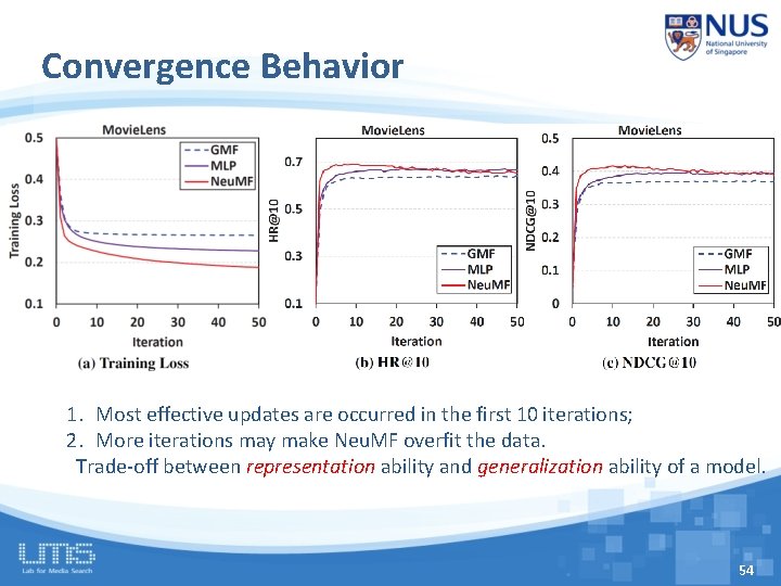
Convergence Behavior 1. Most effective updates are occurred in the first 10 iterations; 2. More iterations may make Neu. MF overfit the data. Trade-off between representation ability and generalization ability of a model. 54

Is Deeper Helpful? 1. Even for models with the same capability (i. e. , same number of predictive factors), stacking more nonlinear layers improves the performance. - Note: stacking linear layers degrades the performance. 2. But the improvement gradually diminishes for more layers - Optimization difficulties (same observation with K. He et al, CVPR 2016) - Residual learning might help. Kaiming He et al. CVPR 2016. “Deep residual learning for image recognition” 55

Conclusion • Most existing recommenders use shallow/linear models. • We explored neural architectures for collaborative filtering. – Devised a general framework NCF; – Presented three instantiations GMF, MLP and Neu. MF. • Experiments show promising results. – Neural nets have good performance in recommendation. – Deeper models are helpful. • Future work: – Tackle the optimization difficulties for deeper NCF models (e. g. , by Residual learning and Highway networks). – Extend NCF to model more rich features, e. g. , user attributes, item description, contextual and temporal signals. 56

Final Thoughts on RS • For RS, academic research has been seldom deployed in industrial use, e. g. : – Taobao mainly uses item-based CF [WWW 2001]. – Linked. In uses linear regression most. – You. Tube used co-view algorithm most. • Deep learning will also overturn the RS area in the next 3 years. – Deep models are much more expressive than past models. – RNNs for temporal modeling: user behaviors are naturally sequential. – There still lacks good DL solutions for sparse data prediction. 57

Thanks! 58