Slides 2 Inventory Management Global Supply Chain Management

Slides 2 Inventory Management Global Supply Chain Management Inventory Management 1

Agenda w Inventory Management Intro w Economic Lot Size Model w Continuous Review Policy w Service level optimization w Risk Pooling / Centralization Inventory Management Slide 2

Inventory Management (IM) w We will introduce here the basics…. w Later, course cases GM, Meditech, Reebok present a diagnosis of a typical problem: low service levels & too high inventory levels. This is actually an Oxymoron…. . w Solutions: co-ordination within or across, better forecasts, reduction of lead time, use Pull, Push-Pull boundaries, postponement. Inventory Management Slide 3

IM implies Order (or Production) Management w Key Question: what, when and how much to order (or: to produce – assume order) w Simple models and principles can provide valuable guidance w At start not like continuous replenishment policy (case of Tesco): we order, the order arrives before we need to order again. Later: orders are underway when we order. Inventory Management Slide 4

Why do we keep Inventory? w Logical: incentives for orders or arriving shipments that are larger (and hence less frequent) compared to leaving sales based on demand: think of a grocery retailer w Uncertainty in supply levels, in lead times w To address uncertainty in demand in combination with long lead times – demand may be hard to forecast, demand may suddenly go up, with high “unsatisfied demand” costs we rather keep some stock, especially if it takes a long time to replenish. w Risks associated with inventories – Shorter lifecycles, more competing products Inventory Management Slide 5

Typical Inventory Policy Factors w w Expectations about customer demand Expectations about lead time Length of the planning horizon (e. g. seasonal ? ) Costs: – Fixed (order) costs, consisting of fixed costs in • Materials and components, storage, admin costs, production costs, transportation costs, Assume that variable costs are covered with sales – Inventory holding costs and associated costs • Taxes and Insurance costs, Maintenance costs • Obsolescence costs and Loss of Opportunity costs w Service level (availability) requirements Inventory Management Slide 6

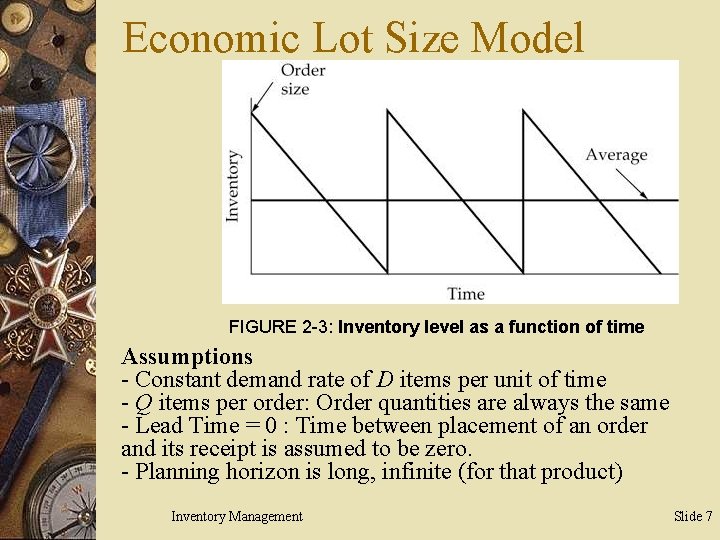
Economic Lot Size Model FIGURE 2 -3: Inventory level as a function of time Assumptions - Constant demand rate of D items per unit of time - Q items per order: Order quantities are always the same - Lead Time = 0 : Time between placement of an order and its receipt is assumed to be zero. - Planning horizon is long, infinite (for that product) Inventory Management Slide 7

Other Assumptions w K fixed setup cost: Every time the warehouse places an order, a fixed setup cost of K is incurred w h inventory carrying cost: A holding cost of h is incurred per unit held in inventory per unit of time w Requested is Q* or EOQ, the Economic Order Quantity Inventory Management Slide 8

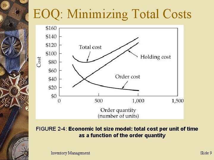
EOQ: Minimizing Total Costs FIGURE 2 -4: Economic lot size model: total cost per unit of time as a function of the order quantity Inventory Management Slide 9

Deriving EOQ w Whatever Q is, at the start of cycle time T we order Q units w The average inventory during a cycle is: Q/2, see diagram w Per T this means a total holding cost of: T * h * Q/2 w For every cycle T we also incur a fixed order cost: K w So the average total cost per cycle: K +T* h *Q/2 w Average total cost per unit of time: K/T + h* Q/2 w Total demand during a cycle is Q = D * T, so T = Q/D w Average total cost per unit of time: K * D/Q + h * Q/2 Inventory Management Slide 10 w This sum of the Order Cost per of unit time and Holding

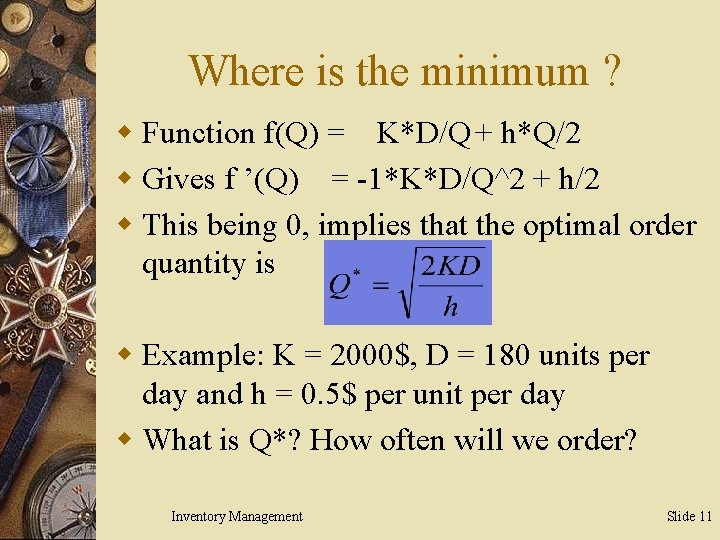
Where is the minimum ? w Function f(Q) = K*D/Q + h*Q/2 w Gives f ’(Q) = -1*K*D/Q^2 + h/2 w This being 0, implies that the optimal order quantity is w Example: K = 2000$, D = 180 units per day and h = 0. 5$ per unit per day w What is Q*? How often will we order? Inventory Management Slide 11

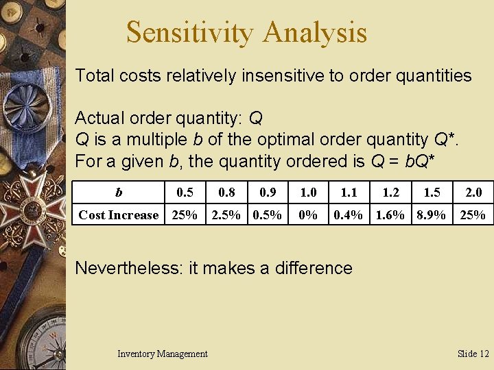
Sensitivity Analysis Total costs relatively insensitive to order quantities Actual order quantity: Q Q is a multiple b of the optimal order quantity Q*. For a given b, the quantity ordered is Q = b. Q* b 0. 5 0. 8 0. 9 Cost Increase 25% 2. 5% 0. 5% 1. 0 0% 1. 1 1. 2 1. 5 2. 0 0. 4% 1. 6% 8. 9% 25% Nevertheless: it makes a difference Inventory Management Slide 12

What if the Manufacturer (or Retailer) has an Initial Inventory? w Trying to use the existing inventory to meet the demand has…. – Advantage: no need to pay production (order) cost – Disadvantage: it may be impossible to meet demand w Producing/ordering on the other hand has…. – Advantage: more likely to meet demand – Disadvantage: implies a production (order) cost, which is relatively high a as we will produce (order) a smaller quantity Inventory Management Slide 13

Multiple Order Opportunities Suppose: demand is uncertain & lead times exist Question: when and how much to order each time? w to balance annual inventory holding costs and annual fixed order costs w to satisfy demand occurring during lead time w to protect against uncertainty in demand Major strategies w Continuous review policy – inventory is continuously reviewed (computerized inventory system) and an order is placed when the inventory reaches a particular level, the reorder point w Periodic review policy (less relevant today) Inventory Management Slide 14

Continuous Review Policy w An entity faces demand according to a normal distribution, the mean demand is AVG and its standard deviation STD. w Every time the entity places an order to its supplier (or decides to manufacture), the entity pays a fixed cost K (plus an amount proportional to the quantity). w Inventory holding cost h is charged per item per unit time. w Inventory level is continuously reviewed, and if an order is placed, the order arrives after the (constant) lead time L. w If customer demand occurs when there is no inventory on hand (i. e. when the entity is stocked out), the order is lost. w The entity specifies a required service level α. This implies that the probability of stocking out during L out is 1 – α. Inventory Management Slide 15

Continuous Review Policy w (Q, R) policy – whenever inventory level falls to a reorder level (point) R, place an order for Q units (optimal order quantity) w What is the optimal value of R? – What is the safety stock level? – What is the demand during the lead time ? w What is the optimal value of Q? w The expected time between orders TBO? w How many inventory turns per unit of time? Inventory Management Slide 16

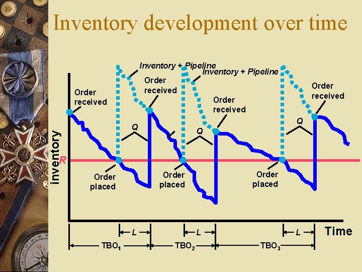
Inventory development over time Inventory + Pipeline Order received inventory Order received Q Q Q R L TBO 1 Order placed L TBO 2 L TBO 3 Time

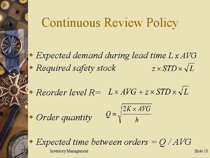
Continuous Review Policy w Expected demand during lead time L x AVG w Required safety stock w Reorder level R= w Order quantity w Expected time between orders = Q / AVG Inventory Management Slide 18

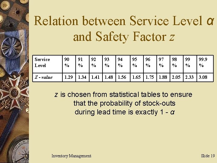
Relation between Service Level α and Safety Factor z Service Level 90 % 91 % 92 % 93 % 94 % 95 % 96 % 97 % Z - value 1. 29 1. 34 1. 41 1. 48 1. 56 1. 65 1. 75 1. 88 98 % 99. 9 % 2. 05 2. 33 3. 08 z is chosen from statistical tables to ensure that the probability of stock-outs during lead time is exactly 1 - α Inventory Management Slide 19

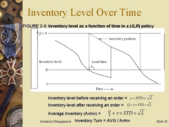
Inventory Level Over Time FIGURE 2 -9: Inventory level as a function of time in a (Q, R) policy Inventory level before receiving an order = Inventory level after receiving an order = Average Inventory (Av. Inv) = Inventory Management Inventory Turn = AVG / Av. Inv Slide 20

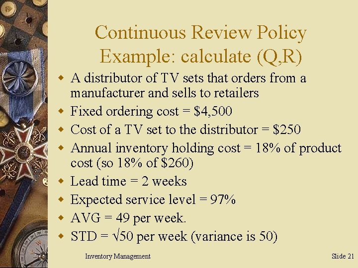
Continuous Review Policy Example: calculate (Q, R) w A distributor of TV sets that orders from a manufacturer and sells to retailers w Fixed ordering cost = $4, 500 w Cost of a TV set to the distributor = $250 w Annual inventory holding cost = 18% of product cost (so 18% of $260) w Lead time = 2 weeks w Expected service level = 97% w AVG = 49 per week. w STD = √ 50 per week (variance is 50) Inventory Management Slide 21

Service Level Optimization w Optimal inventory policy assumes a specific service level target. w What is the appropriate level of service? – May be determined by the downstream customer • The customer may require its supplier (the entity), to maintain a specific service level • The supplier will use that target to manage its own inventory – The Supplier (the Entity) may have the flexibility to choose the appropriate level of service Inventory Management Slide 22

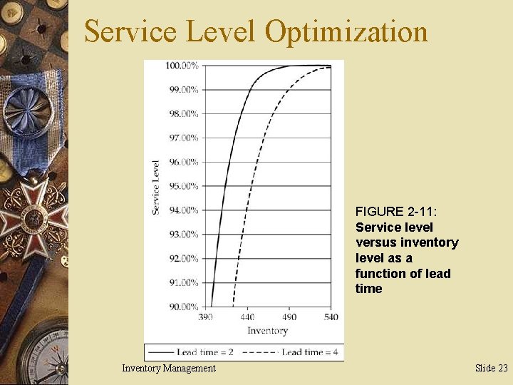
Service Level Optimization FIGURE 2 -11: Service level versus inventory level as a function of lead time Inventory Management Slide 23

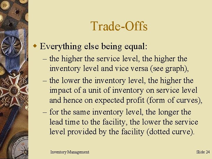
Trade-Offs w Everything else being equal: – the higher the service level, the higher the inventory level and vice versa (see graph), – the lower the inventory level, the higher the impact of a unit of inventory on service level and hence on expected profit (form of curves), – for the same inventory level, the longer the lead time to the facility, the lower the service level provided by the facility (dotted curve). Inventory Management Slide 24

Defining a Retail Strategy w Given a target overall service level across all products w Determine the service level for each SKU so as to maximize expected profit w Everything else being equal, service level will be higher for products with: – – high profit margin high volume low variability short lead time Inventory Management Slide 25

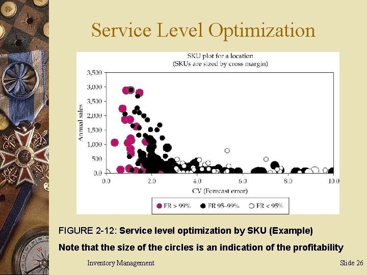
Service Level Optimization FIGURE 2 -12: Service level optimization by SKU (Example) Note that the size of the circles is an indication of the profitability Inventory Management Slide 26

Profit Optimization w A target service level of 97% across all products combined typically leads to a: – Service level > 99% for products with high profit margin, high volume, low variability. – Service level < 95% for products with low profit margin, low volume and high variability. Inventory Management Slide 27

Risk Pooling (based on location) w Demand variability is reduced if one aggregates demand across locations. w More likely that high demand from one customer will be offset by low demand from another customer. w Reduction in variability allows a decrease in safety stock and therefore reduces average inventory. w Other RP factors are time and product Inventory Management Slide 28