Slide for adjusting the presenter position Start of

Slide for adjusting the presenter position

Start of new take Cut after this slide

Maximum likelihood estimation with numerical optimization

Why should an applied researcher care?

Likelihood function Value Likelihood Cumulative likelihood Log likelihood 2 0. 2420000 -1. 419 -1. 42 3 0. 399 0. 0965000 -0. 919 -2. 34 4 0. 242 0. 0234000 -1. 419 -3. 76 Concave function Mean estimated, variance fixed at one Cumulative log likelihood

Finding the maximum bisection method 0 2. 5 2. 97 3. 12 3. 75 2. 81 5

Newton’s method (Newton-Rhapson) Yihui Xie (2013). animation: An R Package for Creating Animations and Demonstrating Statistical Methods. Journal of Statistical Software, 53(1), 1 -27. URL http: //www. jstatsoft. org/v 53/i 01/.

Newton’s method (Newton-Rhapson) Yihui Xie (2013). animation: An R Package for Creating Animations and Demonstrating Statistical Methods. Journal of Statistical Software, 53(1), 1 -27. URL http: //www. jstatsoft. org/v 53/i 01/.

Newton’s method (Newton-Rhapson) Yihui Xie (2013). animation: An R Package for Creating Animations and Demonstrating Statistical Methods. Journal of Statistical Software, 53(1), 1 -27. URL http: //www. jstatsoft. org/v 53/i 01/.

Newton’s method (Newton-Rhapson) When maximizing: With multiple parameters: First derivative Gradient vector Second derivative Hessian matrix Convergence Yihui Xie (2013). animation: An R Package for Creating Animations and Demonstrating Statistical Methods. Journal of Statistical Software, 53(1), 1 -27. URL http: //www. jstatsoft. org/v 53/i 01/.

Newton’s method can fail Yihui Xie (2013). animation: An R Package for Creating Animations and Demonstrating Statistical Methods. Journal of Statistical Software, 53(1), 1 -27. URL http: //www. jstatsoft. org/v 53/i 01/.

Newton’s method can fail Yihui Xie (2013). animation: An R Package for Creating Animations and Demonstrating Statistical Methods. Journal of Statistical Software, 53(1), 1 -27. URL http: //www. jstatsoft. org/v 53/i 01/.

Newton’s method can fail Yihui Xie (2013). animation: An R Package for Creating Animations and Demonstrating Statistical Methods. Journal of Statistical Software, 53(1), 1 -27. URL http: //www. jstatsoft. org/v 53/i 01/.

Newton’s method can fail Yihui Xie (2013). animation: An R Package for Creating Animations and Demonstrating Statistical Methods. Journal of Statistical Software, 53(1), 1 -27. URL http: //www. jstatsoft. org/v 53/i 01/.

Likelihood function What if we estimate both mean and SD? Value Likelihood Cumulative likelihood Log likelihood Cumulative log likelihood 2 0. 2420000 -1. 419 -1. 42 3 0. 399 0. 0965000 -0. 919 -2. 34 4 0. 242 0. 0234000 -1. 419 -3. 76

Numerical optimization of two-variable case

Numerical optimization of two-variable case 136 iterations Newton-Rhapson

Numerical optimization of two-variable case 11 iterations BFGS algorithm with numerical derivatives

Numerical optimization of two-variable case 138 iterations BFGS algorithm with numerical derivatives

Gradient and hessian mean Gradient vector Hessian matrix

Gradient and hessian mean Gradient vector Hessian matrix

Gradient and hessian mean Gradient vector Hessian matrix

Gradient and hessian Gradient vector Hessian matrix

Reasons for convergence problems and possible solutions Problem Solutions Optimization algorithm fails Different algorithm Better starting values Likelihood or derivatives cannot be calculated Different algorithm Better starting values Computer implementation fails Different algorithm Better starting values Different software Not enough iterations Different algorithm Better starting values More iterations Maximum does not exist Modify model Collect more data Solution is not unique (model not identified) Modify model Solution is not unique (empirical underidentification) Modify model Collect more data

End of a good take Cut before this slide

Start of new take Cut after this slide

Hessian matrix in maximum likelihood estimation

Why should an applied researcher care?

Finding the maximum of likelihood

Newton’s method (Newton-Rhapson) When maximizing: With multiple parameters: First derivative Gradient vector Second derivative Hessian matrix Convergence Yihui Xie (2013). animation: An R Package for Creating Animations and Demonstrating Statistical Methods. Journal of Statistical Software, 53(1), 1 -27. URL http: //www. jstatsoft. org/v 53/i 01/.

Convex and concave functions Convex Strictly convex Concave Strictly concave ≥ 0 >0 ≤ 0 <0 Maximum, concave Not concave Neither convex nor concave

Gradient and hessian Gradient vector Hessian matrix

Newton’s method in matrix form •

Newton’s method in matrix form • Distance Direction and distance

Newton’s method in matrix form • If f is steep with respect to m, adjust m more If f curves heavily with respect to s, adjust m more Both equal 0 at convergence Direction for mean Direction for sd Distance Direction and distance If slope of f with respect to m decreases with s, adjust m less If f is steep with respect to s, adjust m less

Convex and concave functions Convex Strictly convex Concave Strictly concave ≥ 0 >0 ≤ 0 <0 ≥ 0 >0 Positive semidefinite Positive definite Negative semidefinite Negative definite ≥ 0 >0 ≤ 0 <0

Convex and concave functions Convex Strictly convex Concave Strictly concave ≥ 0 >0 ≤ 0 <0 ≥ 0 >0 Positive semidefinite Positive definite Negative semidefinite Negative definite ≥ 0 >0 ≤ 0 <0

Negative definite: Diagonal elements are negative and off-diagonal zero

Negative definite: Diagonal elements are negative and off-diagonal zero

Not negative definite: Some diagonal elements non-negative and off-diagonal zero s is not identified

Not negative definite: Some diagonal elements non-negative and off-diagonal zero Saddle point

Convex and concave functions Diagonal elements should be negative Convex Strictly convex Concave Strictly concave ≥ 0 >0 ≤ 0 <0 ≥ 0 >0 Positive semidefinite Positive definite Negative semidefinite Negative definite ≥ 0 >0 ≤ 0 <0 Possible identification problem

Negative definite: Diagonal elements are negative and off-diagonal non-zero

Negative definite: Diagonal elements are negative and off-diagonal non-zero Sign of the off-diagonal elements is not important

Not negative definite: Diagonal elements are negative and off-diagonal non-zero s and m are not identified e. g. estimate: mean(x) = s + m, sd(x) = 1 Absolute value of the off-diagonal element large enough to make the function flat or curve up

Not negative definite: Diagonal elements are negative and off-diagonal non-zero

Not negative definite: Diagonal elements are negative and off-diagonal non-zero

Convex and concave functions Convex Strictly convex Concave Strictly concave ≥ 0 >0 ≤ 0 <0 ≥ 0 >0 Are the off-diagonal elements large enough to make the surface flat or bend it up? Positive semidefinite Positive definite Negative semidefinite Negative definite ≥ 0 >0 ≤ 0 <0 Possible identification problem

What should an applied researcher do? 1. Important to check the last iteration 2. Print out gradient and Hessian 3. Is gradient all zeros? 4. Are the diagonal elements of Hessian all negative 5. Are any of the offdiagonal elements large in absolute value compared to the diagonal elements Note: some statistical software minimize negative log likelihood

End of a good take Cut before this slide

Start of new take Cut after this slide

Matrix algebra

Why should an applied resercher care about matrices? • Reason 1: Understanding books about methods • Reason 2: Matrices are convenient or required for certain calculations • Calculating model implied correlations • Generating simulated dataset • Exporting results as matrices for reproducibility Wooldridge, J. M. (2002). Econometric analysis of cross section and panel data. The MIT Press, p. 189 -190

Diagonal Upper triangle Symmetric matrix Square matrix: m=n Lower tringle Notation: • a – scalar – lower case not bold • a – vector – lower case bolded • A – matrix – upper case bolded Wooldridge, J. M. (2013). Introductory econometrics: A modern approach (5 th ed). South-Western Cengage Learning.

Wooldridge, J. M. (2013). Introductory econometrics: A modern approach (5 th ed). South-Western Cengage Learning.

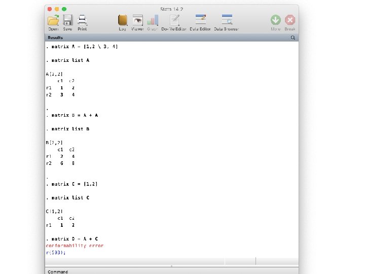
Useful matrix operations to know • Transpose • Addition • Multiplication • Inverse • Determinant

Wooldridge, J. M. (2013). Introductory econometrics: A modern approach (5 th ed). South-Western Cengage Learning.

Wooldridge, J. M. (2013). Introductory econometrics: A modern approach (5 th ed). South-Western Cengage Learning.

Wooldridge, J. M. (2013). Introductory econometrics: A modern approach (5 th ed). South-Western Cengage Learning.

Dimensions of new matrix Must be same 3× 2 3× 3 2× 3

Dimensions of new matrix Must be same 3× 2 3× 3 2× 3

3× 3 3× 2 2× 3

3× 3 3× 2 2× 3

3× 3 3× 2 2× 3

3× 3 3× 2 2× 3

3× 3 3× 2 2× 3

3× 3 3× 2 2× 3

3× 3 3× 2 2× 3

Model implied covariances x 1 x 2 y 1 u 1 y 2 u 2

Model implied covariances x 1 x 2 y 1 u 1 y 2 u 2

Model implied covariances x 1 x 2 y 1 u 1 y 2 u 2 x 1 x 2 y 1 y 2

Matrices: Scalars: Wooldridge, J. M. (2013). Introductory econometrics: A modern approach (5 th ed). South-Western Cengage Learning.

Linear regression in matrix form Wooldridge, J. M. (2013). Introductory econometrics: A modern approach (5 th ed). South-Western Cengage Learning.

What’s the meaning of these equations? Wooldridge, J. M. (2013). Introductory econometrics: A modern approach (5 th ed). South-Western Cengage Learning.

Cross-product matrix X’X n observations • k variables n observations k variables Assume that all variables are centered

Cross-product matrix X’X •

Cross-product matrix X’X • Zero

Cross-product matrix X’X • Scaled version of the covariance matrix

~Covariances between X and e Error term ~Model implied covariances Fitted values ~Observed covariances Wooldridge, J. M. (2013). Introductory econometrics: A modern approach (5 th ed). South-Western Cengage Learning.

This is the equation that the computer uses Wooldridge, J. M. (2013). Introductory econometrics: A modern approach (5 th ed). South-Western Cengage Learning.

Determinant Cannot divide by 0 Distance from 0 • 1. 5 -2 -1 0 1 Area = Determinant x y Linear dependency: One vector can be expressed as weighted sum of others Cannot invert matrix if determinant =0 2

Useful matrix operations to know • Transpose • Addition • Multiplication • Inverse • Determinant

End of a good take Cut before this slide

Start of new take Cut after this slide

End of a good take Cut before this slide